4.5: The Normal Distribution

Last updated
Save as PDF

Page ID: 107470

Maxie Inigo, Jennifer Jameson, Kathryn Kozak, Maya Lanzetta, & Kim Sonier
Coconino Community College

$ \newcommand{\vecs}[1]{\overset { \scriptstyle \rightharpoonup} {\mathbf{#1}} } $ $ \newcommand{\vecd}[1]{\overset{-\!-\!\rightharpoonup}{\vphantom{a}\smash {#1}}} $$\newcommand{\id}{\mathrm{id}}$ $ \newcommand{\Span}{\mathrm{span}}$ $ \newcommand{\kernel}{\mathrm{null}\,}$ $ \newcommand{\range}{\mathrm{range}\,}$ $ \newcommand{\RealPart}{\mathrm{Re}}$ $ \newcommand{\ImaginaryPart}{\mathrm{Im}}$ $ \newcommand{\Argument}{\mathrm{Arg}}$ $ \newcommand{\norm}[1]{\| #1 \|}$ $ \newcommand{\inner}[2]{\langle #1, #2 \rangle}$ $ \newcommand{\Span}{\mathrm{span}}$ $\newcommand{\id}{\mathrm{id}}$ $ \newcommand{\Span}{\mathrm{span}}$ $ \newcommand{\kernel}{\mathrm{null}\,}$ $ \newcommand{\range}{\mathrm{range}\,}$ $ \newcommand{\RealPart}{\mathrm{Re}}$ $ \newcommand{\ImaginaryPart}{\mathrm{Im}}$ $ \newcommand{\Argument}{\mathrm{Arg}}$ $ \newcommand{\norm}[1]{\| #1 \|}$ $ \newcommand{\inner}[2]{\langle #1, #2 \rangle}$ $ \newcommand{\Span}{\mathrm{span}}$$\newcommand{\AA}{\unicode[.8,0]{x212B}}$

There are many different shapes of distributions of quantitative data. In Section 4.2, we examined how a data set was distributed by displaying it in a histogram and frequency polygon. Sometimes the data may have been distributed symmetrically with the highest frequency in the center of the graph while in other instances there appeared to be a higher frequency of data on the left side or right side of the graph.

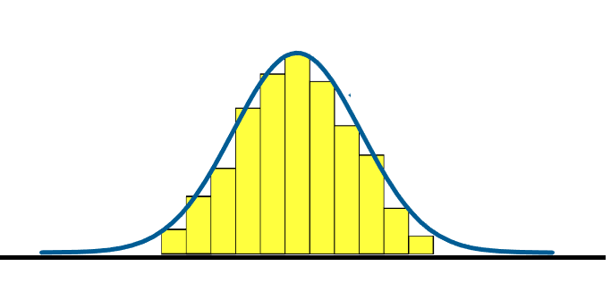
Look at the histogram below where there is a high frequency of data in its middle, and then the frequency goes down quickly and at the same rate as you move away from the middle towards both ends of the histogram. If we "smoothed out" the bars, what's left looks like a bell. This smoothed curve is sometimes called a bell curve.

$A normal curve overlaid on a perfectly symmetric, bell-shaped histogram.$

A wide variety of quantities in the world are distributed in this special way. Given a big enough sample size, a histogram of the sample data would show that the frequency distribution of shoe sizes, IQ scores, life spans of batteries, amounts of coffee distributed by an automatic coffee dispenser, and waiting times for customer service calls, to name a few, all resemble this special distribution.

Moreover, these examples show a typical pattern that seems to be a part of many real-life phenomena. In statistics, because this pattern is so pervasive, it seems fit to call this pattern normal, or more formally, the normal distribution. The normal distribution is an extremely important concept because it occurs so often in data we collect from the natural world, as well as in many of the more theoretical ideas that are the foundation of statistics. Because so many real data sets closely approximate a normal distribution, we can use the idealized normal curve as a model to learn a great deal about such data. In practical data collection, the distribution will never be exactly normal. A true normal distribution only results from an infinite collection of data.

This section explores the basic properties of the normal distribution.

Characteristics of the Normal Distribution

There are several important characteristics that are true about any data that follows a normal distribution.

Shape

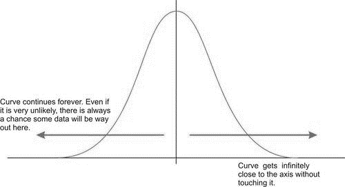
When the data from each of the situations described in the introduction are graphed, the distributions would be mound-shaped and symmetric. A normal model is an idealized, perfectly symmetric, unimodal distribution. In its perfect form, a normal curve extends forever leftwards to $-\infty$ and forever rightwards to $+\infty$. The normal curve is asymptotic to the $x$-axis. That is, the curve gets shorter and shorter as you move left or right along the $x$-axis, but the curve never touches the axis. This indicates that the frequency of observing a data value decreases to almost, but not quite, 0 as you move away from the center of the curve.

$Normal curve with descriptions: An arrow points towards the left side of the curve. Curve continues forever. Even if it is very unlikely, there is always a chance some data will be way out here. An arrow points towards the right side of the curve: Curve gets infinitely close to the axis without touching it.$

Center

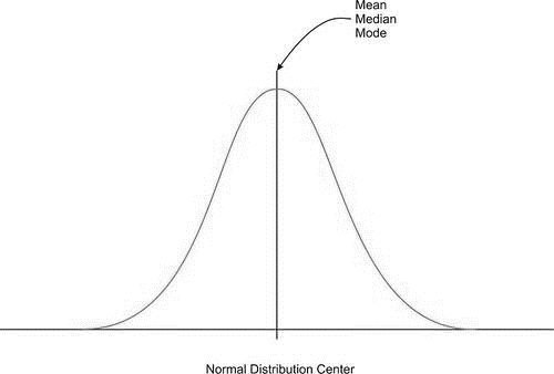
Due to the exact symmetry of a normal curve, the center lies directly below the highest point of the distribution, and all the statistical measures of center we have already studied (the mean, median, and mode) are equal. The symbol we use to represent the mean of a normal curve is the Greek letter $\mu$.

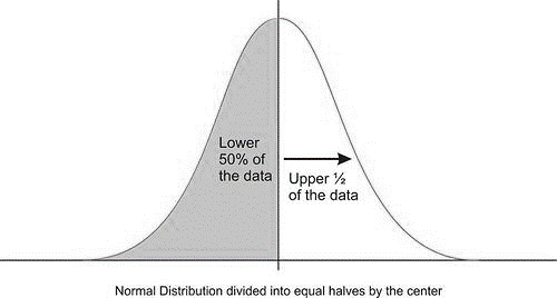
$A normal curve showing the location of the mean, median, and mode all fall directly below the peak.$

It is also important to realize that this location divides the data into two equal parts and corresponds to the 50^th percentile.

$A normal curve split right down the center. On the left side, lower 50% of the data. On the right side, upper 1/2 of the data.$

Spread

Because of the infinite spread of a normal model, the range would not be a useful statistical measure of spread. The most common way to measure the spread of a normal distribution is with standard deviation as the typical distance away from the mean. We use the Greek letter $\sigma$ to represent standard deviation.

Below are two normal distributions. Both have the same mean $\mu= 0$, but they have different standard deviations. Look at how they differ.

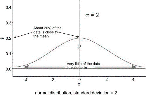
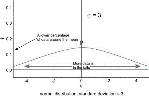
$This is a normal curve with mean 0 and standard deviation 2. The x-axis is labeled x and extends from -4 to 4 in increments of 2. The y-axis extends from 0 to 0.4 in increments of 0.1. The center of the normal curve is over 0 on the x-axis. The peak of the normal curve reaches to a height of about 0.2. About 20% of the data is close to the mean. Very little of the data is in the tails.$ $This is a normal curve with mean 0 and standard deviation 3. The x-axis is labeled x and extends from -4 to 4 in increments of 2. The y-axis extends from 0 to 0.4 in increments of 0.1. The center of the normal curve is over 0 on the x-axis. The peak of the normal curve reaches to a height of about 0.12. A lower percentage of the data around the mean. More data is in the tails.$

The distribution pictured on the left has a smaller standard deviation, and so more of the data are heavily concentrated around the mean than in the distribution on the right. Also, in the first distribution, there are fewer data values at the extremes than in the second distribution. Because the second distribution has a larger standard deviation, the data are spread farther from the mean value, with more of the data appearing in the tails.

The Empirical Rule

Another property of the normal distribution has to do with the relative frequency of data that falls within a given distance from the mean. And since empirical probability is nothing more than relative frequency, we can also consider this property to tell us about the probability that a certain value falls within a given distance from the mean.

The Empirical Rule is a property that holds for all normal curves and can be used as a guide to approximate relative frequencies and probabilities for certain intervals of the normal curve. The Empirical Rule is also known as the 68-95-99.7 Rule for reasons that will be obvious.

The Empirical Rule for Normal Distributions
Approximately 68% of the outcomes are within one standard deviation of the mean.	$P(\mu - \sigma < X < \mu + \sigma)$
Approximately 95% of the outcomes are within two standard deviations of the mean.	$P(\mu - 2\sigma < X < \mu + 2\sigma)$
Approximately 99.7% of the outcomes are within three standard deviations of the mean.	$P(\mu - 3\sigma< X < \mu + 3\sigma)$

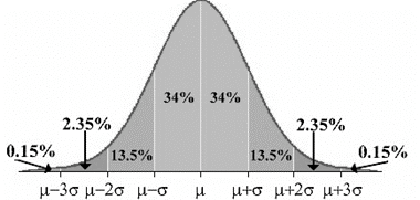
$A normal curve showing the percentages of the Empirical Rule. 68% of the data lies within 1 standard deviation of the mean. 95% of the data lies within 2 standard deviations of the mean. 99.7% of the data lies within 3 standard deviations of the mean.$

Be careful: There is still a portion of the normal curve left over in each end beyond $\mu-3\sigma$ and $\mu+3\sigma$. The total relative frequency for the entire distribution is 100%. If you calculate $100\% - 99.7\%$ you will see that for both ends together there is $0.3\%$ of the data remaining. Because of symmetry, you can divide this equally between both ends and find that there is $0.15\%$ in each tail beyond $\mu \pm 3\sigma$. Here is a more detailed picture of the percentages in each of the eight intervals created when counting 3 standard deviations on each side of the mean:

$A normal curve showing percentages of data under the normal curve between each interval of sigma. From left to right, the percentages are 0.15%, 2.35%, 16%, 34%, 34%, 16%, 2.35%, and 0.15%.$

The Empirical Rule is effective to use only when we have endpoints of the interval that are exactly 1, 2, or 3 standard deviations from the mean. If we want to find percentages or probabilities involving values of $X$ that are not integer multiples of the standard deviation, we will need to use technology as shown further in this section.

Let's consider some scenarios where we can apply the Empirical Rule.

Example 1

The mean and standard deviation for the age when a child starts walking are 15 months and 3 months, respectively. Assume $X$, the age at which children first walk, is normally distributed.

What percent of children start walking between 12 and 18 months of age?

The Empirical Rule can be used because the problem states that $X$ follows a normal distribution. Start with a picture that relates the percentages and the values of the mean and standard deviation. In the problem we are given that $\mu=15$ and $\sigma = 5$.

$A normal curve with x-axis labeled from 6 to 24 in increments of 3 showing percentages of data under the normal curve between each interval of sigma. From left to right, the percentages are 0.15%, 2.35%, 16%, 34%, 34%, 16%, 2.35%, and 0.15%.$

Looking at the portion of the curve from $X=12$ to $X =18$, we can combine the percentages shown in the middle two sections of the normal curve to find the total percentage: $P(12 < X < 18)= 34\%+34\%=68\%$.

We can say that about 68% of all children walk for the first time when they are between the ages of 12 and 18 months.

What percentage of children walk for the first time before age 18 months?

Using the same picture from part a, we can add the percentages to the left of $X=18$. One way to do this is to add the area of each section separately: $P(X<18)= 0.15\% + 2.35\% +13.5\% +34\% +34\% = 68\%$.

You could also add the percentage left of the mean ($50\%$) to the percentage from the mean $\mu$ to $\mu + \sigma$ ($34\%$) to get $84\%$.

About $84\%$ of children walk for the first time before 18 months of age.

Approximate the percentage of children who start walking after 21 months of age.

Using the same picture from part a, we can add the percentages to the right of $X=21$: $2.35\% + 0.15\% = 2.5\%$. About 2.5% of all children first walk after they are 21 months old.

Example 2

Your class took a test and the mean score was 75 points and the standard deviation was 5 points. The test scores follow an approximately normal distribution. Sketch a normal curve and use it to answer these questions.

What percentage of the students had scores between 65 and 85?
What percentage of the students had scores between 65 and 75?
What percentage of the students had scores between 70 and 80?
What percentage of the students had scores above 85?

Solution

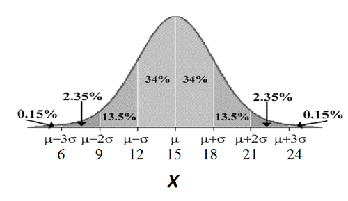
To solve each of these questions, it would be helpful to draw the normal curve that represents this situation. The mean is 75, so place 75 below the peak. The standard deviation is 5, so to label the axis, add 5 to the mean 3 times and subtract 5 from the mean 3 times. The graph looks like the following:

$A blank normal curve with the x-axis labeled from 55 to 95 in increments of 5.$

From the graph, $X = 65$ and $X=85$ are both two standard deviations from the mean. According to the Empirical Rule, this percentage must be $95\%$..
The scores from $X = 65$ to $X = 75$ make up half of the percentage from $X=65$ to $X=85$. Because of symmetry, that means that $P(65 < X < 75$ is ½ of the answer to part a: $\frac{1}{2} \times 95\% = 47.5\%$. You could have also added $13.5\% + 34\%$.
From the graph, $X = 70$ and $X=80$ are both one standard deviation from the mean. According to the Empirical Rule, this percentage must be $68\%$.
One way to find $P(X>85)$ is to add $2.35\% + 0.015\% = 2.5\%$. There are other strategies too.

Try it Now 1

The distribution of wait times at a drive-through restaurant is approximately normal with mean 185 seconds and standard deviation 15 seconds. Use a sketch and the Empirical Rule to find the percentage of wait times that are

between 155 and 215 seconds.
more than 170 seconds.
less than 155 seconds.
between 170 and 215 seconds.

Answer

95%
84%
2.5%
81.5%

z-scores

Now we will begin to consider situations when the Empirical Rule cannot be used -- that is, when a value is not exactly one, two, or three standard deviations from the mean.

Let's return to the scenario in Example 1. Suppose we want to know the percentage of children who start walking after 10 months, or $P(X>10)$. Recall the sketch of the normal curve:

The value of $X = 10$ does not fall exactly on any of the numbers we marked on the axis of the normal distribution. It is more than one but less than two standard deviations away from the mean of 15 months. We can compute what is called a z-score to measure how many standard deviations the value $X = 10$ is from the mean.

z-score

A z-score measures how many standard deviations a data value is from the mean of the distribution. To calculate the z-score for a value, find its deviation from the mean and divide by the standard deviation.

The formula for a z-score is $z=\dfrac{x-\mu}{\sigma}$ where

$x$ is the data value (raw score),
$z$ is the standardized value ($z$-score or $z$-value)
$\mu$ is the mean
$\sigma$ is the standard deviation.

For a child that walks at $X = 10$ months, the z-score is $z=\dfrac{x-\mu}{\sigma} = \dfrac{10-15}{3}=\dfrac{-5}{3} \approx -1.67$. This means that this child is about 1.67 standard deviations below the mean age when children first begin to walk.

Using Technology to Find Percentages of a Normal Distribution

Once upon a time, finding percentages using the normal curve involved first computing z-scores and then consulting tables of normal areas in textbooks. Fortunately, as technology has developed to the point where we are now, we can use calculators and computers to find percentages when a variable follows a normal model. We will assume the use of technology in this course, but sketching a picture of the situation is still very useful.

The table below shows the general steps for finding percentages with the TI calculator. Example 3 below will demonstrate use of the steps.

$TI graphing calculator steps to find percentages corresponding to an interval on the normal curve.$

Example 3

Lengths of human pregnancies are normally distributed with a mean $\mu=272$ days and standard deviation $\sigma = 9$ days.

Find the percentage of pregnancies that last more than 280 days.

Translate the question into a mathematical statement and draw a sketch of a normal curve with $\mu=272$ and $\sigma = 9$. Then, use the normalcdf( command. The lower endpoint of the interval is 280 and the upper endpoint of the interval is +∞.

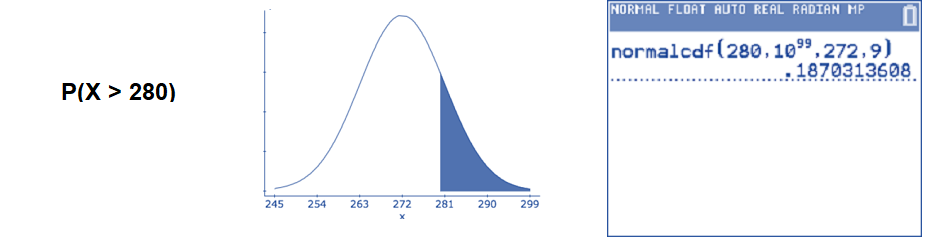
$This is a normal curve with shaded area to the right of 280. A TI graphing calculator screenshot shows normalcdf(280, 10^99, 272, 9) = 0.1870.$

$P(X>280) \approx 0.1870$: We can say that 18.70% of all human pregnancies last more than 280 days.

Find the percentage of pregnancies that last less than 250 days.

Translate the question into a mathematical statement and draw a sketch of a normal curve with $\mu=272$ and $\sigma = 9$. Then, use the normalcdf( command. The lower endpoint of the interval is $-\infty$ and the upper endpoint of the interval is 250.

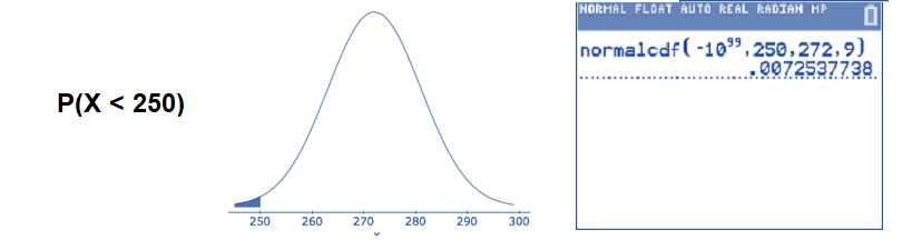
$This is a normal curve with shaded area to the left of 250. A TI graphing calculator screenshot shows normalcdf(-10^99, 250, 272, 9) = 0.0073..$

$P(X<250) \approx 0.0073$: We can say that 0.75% of all human pregnancies last less than 250 days. This appears to be quite unusual.

Find the percentage of pregnancies that last between 265 and 280 days.

$This is a normal curve with shaded area between 265 and 280. A TI graphing calculator screenshot shows normalcdf(265, 280, 272, 9) = 0.5946.$

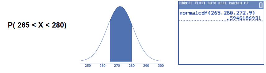
$P(265<X<280) \approx 0.5946$: About 59.46% of all human pregnancies last between 265 and 280 days.

Example 4

The mean score on a reading test for 4^th graders is 514 points with standard deviation 117 points. Assume that scores on this test are normally distributed.

Find the percentage of students who score at least 700 on this test.

The question asks for the percentage to the right side of 700. Recall that 'at least' means 700 or more. Translate the problem into a mathematical statement, draw a picture, and use the Normalcdf( command on the TI calculator.

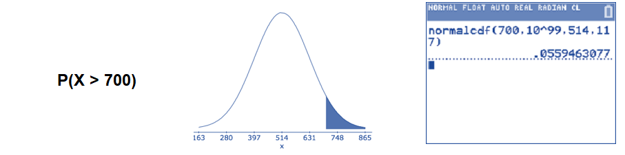
$This is a normal curve with shaded area to the right of 700. A TI graphing calculator screenshot shows normalcdf(700, 10^99, 514, 117) = 0.0559.$

$P(X>700) \approx 0.0559$: About 5.59% of 4^th graders scored at least 700 on the reading test.

What percentage of 4^th graders score less than 400 on the reading test?

This asks for the percentage to the left side of 400. Use the normalcdf( command.

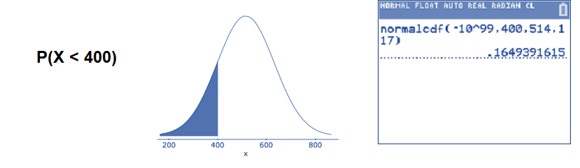
$This is a normal curve with shaded area to the left of 400. A TI graphing calculator screenshot shows normalcdf(-10^99, 400, 514, 117) = 0.1649.$

$P(X<400) \approx 0.1649$: Approximately 16.49% of 4^th graders scored less than 400 on this reading test.

Find the percentage of 4^th graders who score between 500 and 650.
The question asks for the percentage between 500 and 600. Use the normalcdf( command.

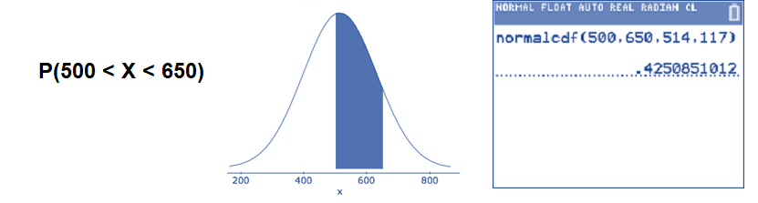
$This is a normal curve with shaded area between 500 and 650. A TI graphing calculator screenshot shows normalcdf(500, 650, 514, 117) = 0.4251.$

$P(500<X<650) \approx 0.4251$: The percentage of 4^th graders with scores between 500 and 650 is approximately 42.51%.

Try it Now 2

The average amount of caffeine consumed daily by an adult is normally distributed with mean of 250 mg and standard deviation of 48 mg.

Use technology to find the percentage of adults who consume these amounts of caffeine daily:
1. more than 310 mg.
2. less than 250 mg.
3. between 202 mg and 346 mg.
4. more than 400 mg.
In a random sample of 500 adults, how many should consume at least 310 mg?

Answer

i. 10.56% ii. 50% iii. 81.86% iv. 0.09%
53 adults

Using Technology to Find a Value from a Normal Distribution

In Example 3 we found the relative frequency of pregnancies that lie within a particular interval. All the questions in Example 3 asked for a percentage when given intervals of values for $X$ such as $P(X >280)$, $P(X<250)$, or $P(165<X<280)$. When we were given a value of the variable and were asked to find the percentage, we used the normalcdf( command on the TI calculator.

Now, we will consider the reverse operation. In other words, we will be concerned with finding a value for $X$ that cuts off a given relative frequency on its left side or on its right side. Again, the TI calculator is convenient and accurate. The command on the TI calculator for this process is invNorm(. You may have seen it already in the Distribution menu.

Example 5

Revisiting the scenario from Example 3, lengths of human pregnancies are normally distributed with a mean $\mu=272$ days and standard deviation $\sigma = 9$ days. Find the lengths of the shortest 10% of pregnancies.

Solution

The question asks for an $X$-value in the normal distribution. You want to locate the $X$-value on the axis that has 10% of pregnancies to the left of it. Translate the problem into a mathematical statement and make a sketch showing that the area to left of some unknown $X$ is 0.10. Then, use the invnorm( command with left-sided area 0.10.

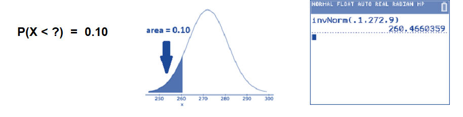
$This is a normal curve with left side shaded that has an area of 0.10. A TI graphing calculator screenshot shows invnorm(0.10, 272, 9) = 260.47.$

Thus, 10% of all human pregnancies last less than about 260 days. We could also say that 90% of all human pregnancies last longer than 260 days. The value $X=260$ separates the shortest 10% of human pregnancies from the longest 90%. As you may recall from an earlier section, we call 260 days the 10^th percentile.

If we had wanted to find the longest 10% of pregnancies instead, we would have used the same command. But, we need to be careful about choosing the correct side of the normal curve.

For the longest 10% of pregnancies, we want to find the value for $X$ so that $P(X>?=0.10$. Depending on the calculator version, you may be able to specify that you want the "right tail." If you don't have the option to choose the right tail, then you must find the $X$-value that cuts off the left 90% from the right 10% in a similar way to what we did in Example 5. Calculator screens for both versions of the calculator are shown.

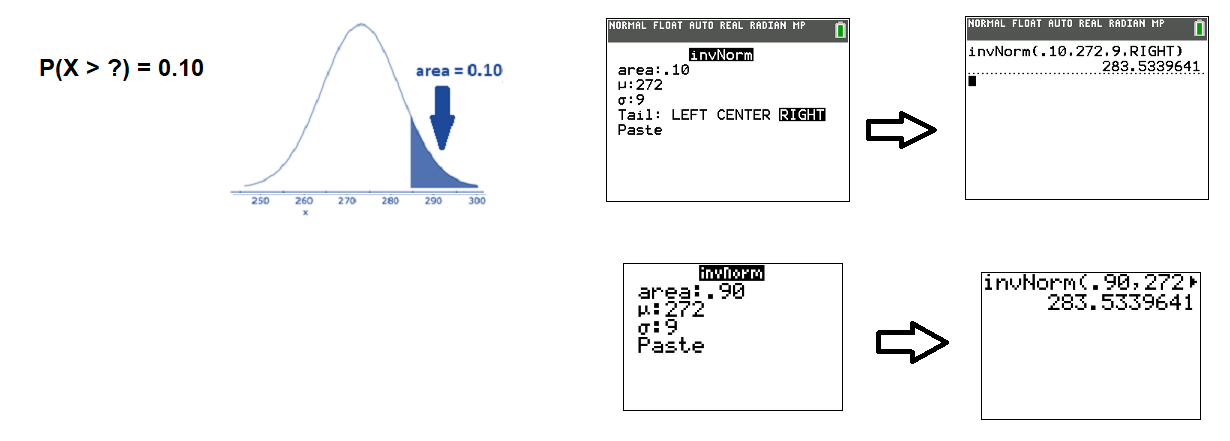
$This is a normal curve with right side shaded that has an area of 0.10. A TI graphing calculator screenshot shows invnorm(0.10, 272, 9, right) = 283.53.$

Thus, 10% of all human pregnancies last longer than about 284 days. We could also say that 90% of all human pregnancies are shorter than 284 days. The value $X=2$84 separates the shortest 90% of human pregnancies from the longest 10%. We call 284 days the 90^th percentile.

Example 6

Sarah keeps statistics for the baseball team. Based on her records, the distances that fly balls are hit to the outfield are approximately normally distributed with a mean 250 feet and standard deviation 50 feet.

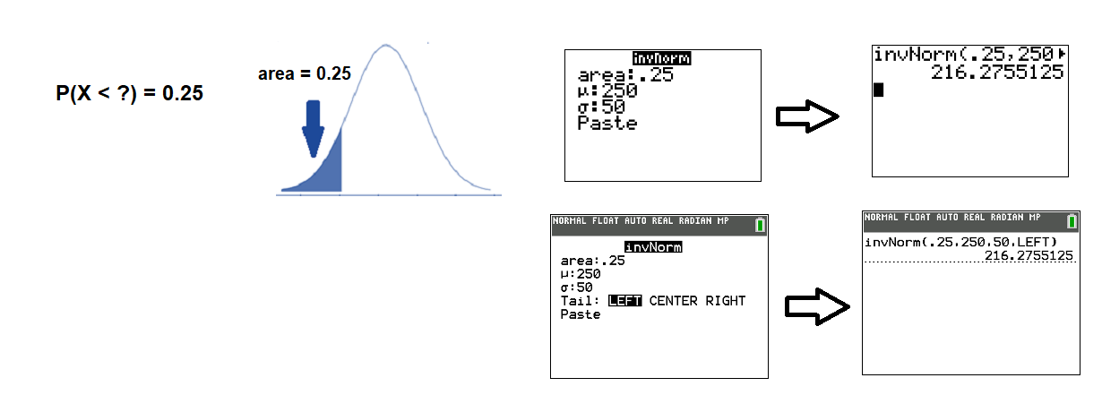
How far are the shortest 25% of all fly balls hit?
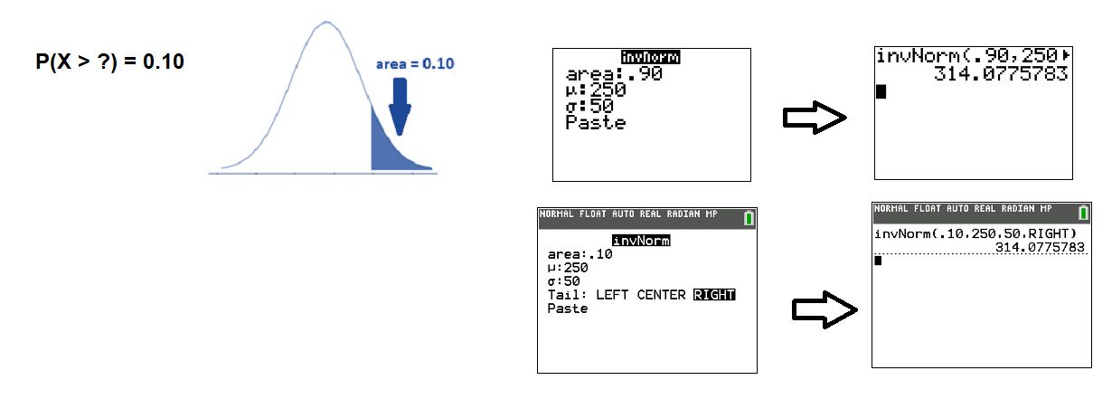
How far will a player need to hit a fly ball for it to be in the top 10% of all fly balls that are hit?

Solution

We want to find the $X$-value so that 25% of fly ball distances are lower than $X$. This means the area to the left of $X$ is 0.25. As the calculator screen shows, the shortest 25% of all fly balls travel less than 216 feet.

$This is a normal curve with left side shaded that has an area of 0.25. A TI graphing calculator screenshot shows invnorm(0.25, 250, 50, left) = 216.28$

We want to find the $X$-value so that 10% of fly ball distances are greater that $X$. This means the area to the right of $X$ is 0.10. As the calculator screen shows, a player needs to hit the fly ball a distance of 314 feet or more.

$This is a normal curve with right side shaded that has an area of 0.10. A TI graphing calculator screenshot shows invnorm(0.10, 250, 50, right) = 314.08.$

Try it Now 3

A citrus farmer who grows tangerines finds that the diameters of tangerines harvested on his farm follow a normal distribution with a mean diameter 5.85 cm and standard deviation of 0.25 cm. Use a TI calculator to complete each statement.

The smallest 15% of tangerines have diameters that measure _____ cm or smaller.
The largest 25% of tangerines have diameters that measure _____ cm or bigger.

Answer

5.59
6.02

Approximately 68% of the outcomes are within one standard deviation of the mean.	\(P(\mu - \sigma < X < \mu + \sigma)\)
Approximately 95% of the outcomes are within two standard deviations of the mean.	\(P(\mu - 2\sigma < X < \mu + 2\sigma)\)
Approximately 99.7% of the outcomes are within three standard deviations of the mean.	\(P(\mu - 3\sigma< X < \mu + 3\sigma)\)