 Karina Cucchi
 Nicolas Flipo
 Agnès Rivière
 Yoram N. Rubin
- 1Department of Civil and Environmental Engineering, University of California, Berkeley, Berkeley, CA, United States
- 2Geosciences Department, MINES ParisTech, PSL Research University, Paris, France
Located in the critical zone at the intersection between surface water and groundwater, hyporheic zones (HZ) host a variety of hydrological, biological and biogeochemical processes regulating water availability and quality and sustaining riverine ecosystems. However, difficulty in quantifying water fluxes along this interface has limited our understanding of these processes, in particular under dynamic flow conditions where rapid variations can impact large-scale HZ biogeochemical function. In this study, we introduce an innovative measurement assimilation chain for determining uncertainty-quantified hydraulic and thermal HZ properties, as well as associated uncertainty-quantified high-frequency water fluxes. The chain consists in the assimilation of data collected with the LOMOS-mini geophysical device with a process-based, Bayesian approach. The application of this approach on a synthetic case study shows that hydraulic and thermal HZ properties can be estimated from LOMOS-mini measurements, their identifiability depending on the Peclet number – summarizing the hydrological and thermal regime. Hydraulic conductivity values can be estimated with precision when greater than ~10−5m · s−1 when other HZ properties are unknown, with decreasing uncertainty when other HZ properties are known prior to starting the LOMOS-mini measurement assimilation procedure. Water fluxes can be estimated in all regimes with varying accuracy, highest accuracy is reached for fluxes greater than ~10−6m · s−1, except under highly conductive exfiltration regimes. We apply the methodology on in situ datasets by deriving uncertainty-quantified HZ properties and water fluxes for 2 data points collected during field campaigns. This study demonstrates that the LOMOS-mini monitoring technology can be used as complete and stand-alone sampling solution for quantifying water and heat exchanges under dynamic exchange conditions (time resolution < 15 min).
1. Introduction
Sustainable management of surface water and groundwater resources and of the ecosystems they support requires a reliable quantification of stream-aquifer water exchanges (Winter et al., 1998; Woessner, 2000; Stonestrom and Constantz, 2003; Fleckenstein et al., 2010). Indeed, these exchanges condition the water budget of hydrosystems (Krause and Bronstert, 2007), seasonal low flows (Fleckenstein et al., 2006; Kløve et al., 2014) and contaminant transport in the stream-aquifer continuum (Conant, 2004; Lewandowski et al., 2011). Coupled with heat fluxes, water fluxes also condition a myriad of chemical and ecological processes, such as denitrification rates (Harvey et al., 2013; Newcomer et al., 2018), locations of refuge for aquatic species (Brunke and Gonser, 1997; Malcolm et al., 2005; Marmonier et al., 2012) and they play a critical role in maintaining a good quality of stream water (Hancock, 2002).
Located in the critical zone at the transition between surface water and groundwater, the hyporheic zone (HZ) is defined as the subsurface area where water exchanges are driven both by stream pressure gradients and subsurface properties (Tonina and Buffington, 2009; Peralta-Maraver et al., 2018). Water and heat fluxes in the HZ have emerged as having a significant role from the micro scale to the catchment scale (Boulton et al., 1998; Bencala, 2000) and have been increasingly studied in the past decades (e.g., Boano et al., 2014; Flipo et al., 2014; Cardenas, 2015; Brunner et al., 2017; Lewandowski et al., 2019).
A variety of technologies and methods have been proposed to study HZ water exchanges, ranging from seepage meters, chemical or isotopic tracers (e.g., Kalbus et al., 2006; Rosenberry and LaBaugh, 2008; Xie et al., 2016). Amongst them, the use of heat as a tracer is well-established thanks to the relatively low cost of temperature sensors and the ease of deployment (Lapham, 1989; Anderson, 2005; Constantz, 2008; Rau et al., 2014; Kurylyk and Irvine, 2019; Kurylyk et al., 2019). It is enabled by the relative stability of groundwater temperatures, whereas stream temperatures exhibit strong diurnal and annual cycles. The propagation of daily river temperature signals in the hyporheic is particularly sensitive to flow variations because thermal properties are much less variable than hydraulic properties: thermal conductivity ranges between 1.5 and 6 W m−1 °C−1 for unconsolidated water saturated porous materials while hydraulic conductivity can vary over 6 orders of magnitude (e.g., Lapham, 1989; Constantz et al., 2002; Rivière et al., 2020). Various analytical and numerical methods based on the heat transfer equation have emerged (e.g., Stallman, 1965; Hatch et al., 2006; Rau et al., 2014; Irvine et al., 2020). Related software implementations are the VFLUX2 software using the steady state analytical solution (Gordon et al., 2012; Irvine et al., 2015b), the FAST program using the transient analytical solution (Kurylyk and Irvine, 2016), or the FLUX-BOT Matlab program using a numerical model for solving the advection-diffusion equation (Munz and Schmidt, 2017). More recently, the Fiber-Optic Distributed Temperature Sensing (FO-DTS) technology was introduced for hydrological applications, opening new opportunities for inferring patterns of groundwater discharge into streams continuously along the streambed (Selker et al., 2006a,b; Briggs et al., 2012).
Amongst technologies using heat as a tracer for quantifying water exchanges in the HZ, the uniqueness of the LOMOS-mini sensor device resides in the ability to quantify transient exchanges at a high temporal resolution, thereby relaxing the assumption of constant daily exchanges and opening the opportunity to monitor rapid infiltration and exfiltration events at the time scale at which they happen (Cucchi et al., 2018). The technology is based on a coupled approach combining vertically-distributed temperature and pressure differential monitoring (Figure 1), and on a process-based numerical model for estimating water and heat fluxes (where process-based model refers to a mathematical description of physical processes at play, e.g., Clark et al., 2017). The methodology presented to date assumes that hydraulic and thermal properties in the HZ are deterministically known.
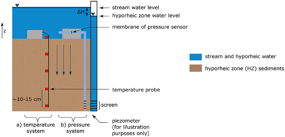
Figure 1. Cross-sectional view of the LOMOS-mini monitoring system. It consists in vertically-distributed temperature sensors (in red) and a hydraulic head difference sensor. Reproduced from Cucchi et al. (2018).
Here we introduce a new application of the LOMOS-mini monitoring technology, where the collected measurements are used for estimating hydrological and thermal properties in the HZ. The approach assimilates vertically-distributed temperature and pressure differential time series measured at a high frequency by the LOMOS-mini sampling device. It uses a Bayesian approach and a process-based forward model for estimating the joint statistical distribution of HZ properties, thereby allowing to investigate the identifiability of HZ properties—that is, the possibility of estimating the true values of underlying HZ properties knowing LOMOS-mini measurements.
Section 2 introduces an application of the Bayesian framework for estimating statistical distributions of HZ hydrogeological and thermal properties from LOMOS-mini measurements. In line with Rivière et al. (2020), section 3 applies the framework on a synthetic case study, investigating parameter identifiability for various hydrological and thermal forcings (exfiltration/infiltration, advective/conductive), as well as for a range of lithofacies. Section 4 applies the framework to in situ measurements collected in the Avenelles basin, France. Section 5 discusses results in the light of alternative sampling solutions, and proposes that the unique value of the introduced method relies in being a complete and stand-alone solution for estimating high-frequency transient water and heat exchanges, as well as associated HZ hydraulic and thermal properties.
2. Methods
This section describes the data assimilation chain developed to estimate HZ properties and high-frequency exchanged fluxes from LOMOS-mini measurements. The data assimilation is posed in a Bayesian framework (section 2.1), relying on the assimilation of in situ LOMOS-mini measurements via a process-based model (section 2.2) and allowing to incorporate any level of previous experience working with HZ unknown properties (section 2.3). Besides the application of Bayesian inference, an innovative feature of the proposed framework is to simplify the estimation problem by noticing that it can be reduced to 2 effective parameters (section 2.2.1), thereby allowing to ease the investigation of the problem and shorten execution times (section 2.2.2). The outcome of this assimilation chain is uncertainty-quantified HZ property estimates, allowing to investigate the extent to which LOMOS-mini measurements allow to characterize HZ properties, as well as uncertainty-quantified water exchanges with a 15 min temporal frequency (section 2.4).
The data assimilation chain and subsequent analyses were implemented with the R statistical software and the tidyverse collection of R packages for data science (Wickham et al., 2019; R Core Team, 2020). We implemented a suite of utility functions specific to our study in the form of an R package (Wickham, 2015), which can be found through a GitHub repository at https://github.com/kcucchi/HZinv.
2.1. Bayesian Data Assimilation
Quantifying water movement in the subsurface generally relies on the interpretation of collected environmental data, and is hindered by a lack of information about subsurface properties due to low data availability as well as spatial and temporal variability. Stochastic hydrogeology provides a framework for assimilating information contained in sparse environmental data by posing problems in a probabilistic yet physical framework. Unknown physical properties y in the subsurface are considered as random variables defined by their probability density function (pdf) fY(y), thereby representing a wide range of states of knowledge, where at one end broad based pdfs fY(y) represent maximum uncertainty and at the other end narrow pdfs represent low uncertainty, with varying degrees of uncertainty in between (Rubin, 2003). Notations in this paper are that uppercase letters represents the random variable and lowercase letters represent their realizations. Physical properties are linked to observations θ* by means of process-based models (Gelhar, 1993; Rubin, 2003). Y and θ* typically have multiple dimensions and are therefore represented using boldface, where boldface denote vectors (Table 1). Here, θ* are LOMOS-mini measurements and Y are unknown HZ properties.
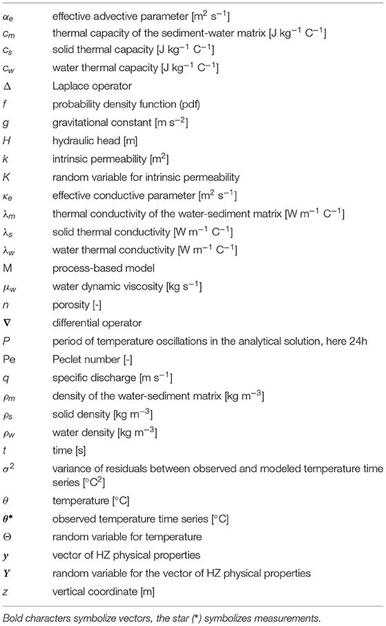
Table 1. Notations.
Bayesian inference uses the information contained in field measurements θ* to improve the characterization of Y. In statistical terms, this means conditioning the pdf fY(y) on the available data θ* that are related to y, by calculating the conditional pdf . The basis of Bayesian inference is Bayes' theorem, which is stated as follows:
fY(y) is the prior pdf, describing model parameters y before accounting for measurements, is the likelihood function describing the discrepancy between and observed data and model predictions with parameters y, and is the posterior pdf describing model parameters once measurements are assimilated.
The prior pdf fY(y) represents the knowledge about the target parameters Y before accounting for data measured in situ, in other words the data measured at the site under investigation (Rubin, 2003). As further detailed in section 2.3, Bayesian inference is flexible in the amount of information to account for prior to starting the assimilation of in situ measurements (Rojas et al., 2009; Kitanidis, 2012; Li et al., 2018; Cucchi et al., 2019; Heße et al., 2021).
The likelihood function links the prior pdf to the posterior pdf. It is defined as the probability of observing measurements θ* conditionally on physical parameters y, where parameters leading to model outputs similar to observations receive high probability (e.g., Tarantola, 2005; Scholer et al., 2012; Anderson and Segall, 2013). Measurements θ* and physical parameters y are linked via a process-based model M, further described in section 2.2. In this study, the likelihood function is formulated as a weighted Gaussian probability density centered around temperature observations θ* (e.g., Scholer et al., 2012) as follows:
where N is the number of sampled points, t is an index referring to the sample in the time series, and σ2 is the variance of the residuals.
The result of the Bayesian inference can then be calculated from the prior distribution and the likelihood function (Equation 2) using Bayes' theorem (Equation 1).
In cases where measurements helped to better characterize the unknown property—i.e., when the posterior distribution is narrow when compared to the prior distribution fY(y)—we refer to Y as being identifiable (e.g., Carrera and Neuman, 1986; Vrugt et al., 2002; Scharnagl et al., 2011). This also corresponds to cases where the likelihood function is narrow when compared to the prior.
2.2. Definition of the Likelihood Function
In this study, the likelihood function is based on a process-based model M linking LOMOS-mini measurements θ* to unknown HZ properties Y. This section presents the mathematical equations used to represent the physical processes at play in the streambed, as well as the adopted analytical and numerical solutions.
2.2.1. Physical Conceptualization
The heat equation simulates heat transport in porous media:
where θ [°C] represents temperature, ρm [kg m−3] is the density of the sediment-water matrix, cm [J kg−1 °C−1] is the specific heat capacity of the sediment-water matrix, ρw [kg m−3] is the water density, cw [J kg−1 °C−1] is the water specific heat capacity, and λm [W m−1 °C−1] is the bulk thermal conductivity. ∇ is the differential operator and Δ is the Laplace operator. q is the specific discharge [m s−1], it represents the water flux through a unit cross-sectional area normal to the direction of flow (e.g., Bear, 1979; de Marsily, 1986). Notations are summarized (Table 1).
q and k are linked by Darcy's law:
where k [m2] is the intrinsic permeability, g [m s−2] is the gravitational constant, and μw [kg s−1] is the water dynamic viscosity.
λm is the thermal conductivity of the water-sediment matrix and is modeled to be linked to the water and sediment thermal conductivities λw and λs via a functional relationship as discussed below. Several models have been proposed, here we follow the recommendation of Cosenza et al. (2003) as it is done in the numerical code Ginette (Rivière et al., 2014, 2019) and use the quadratic parallel formulation:
In this study, we neglect thermal dispersion. The formulation of the dispersion term and its influence on heat transport at different spatial and temporal scales is questioned in the literature and is unsolved to date (Rau et al., 2014). In similar studies, the dispersion is usually neglected and justified given the small spatial extent and small specific discharge in the experimental setting (Silliman et al., 1995; Luce et al., 2013).
While values of certain physical properties are deterministically known, other ones vary depending on geological environments at investigated locations and are therefore modeled as stochastic random variables. Table 2 summarizes parameters, indicating which are known deterministically and which are modeled stochastically, with associated numerical values or physically plausible variation ranges. The vector of unknown physical properties modeled as random variables is Y = (n, ρs, cs, λs, k).
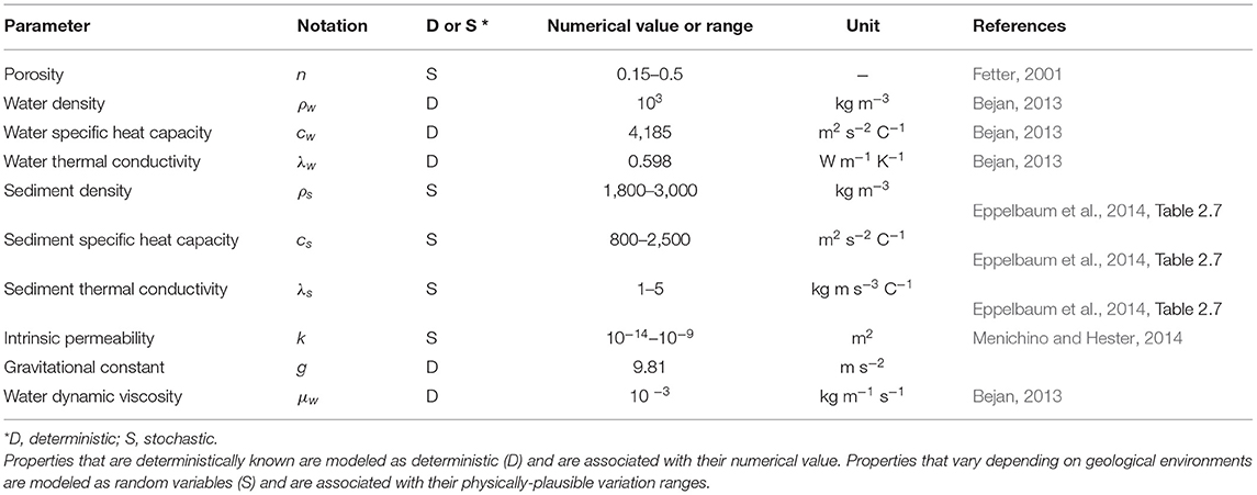
Table 2. HZ properties in the process-based model.
Finally, it is worth noticing that while there are 5 unknown HZ properties in vector y, there are only 2 degrees of freedom in the physical system. Indeed, the ADE (Equation 3) and the flow equation (Equation 4) can be merged into a single equation as follows:
κe [m2 s−1] and αe [m s−1] are effective parameters of the problem and function of physical properties in Table 2. In this study, we refer to κe and αe as effective conductive and effective advective parameters respectively. κe is also known as effective thermal diffusivity (e.g., Suzuki, 1960).
For every set of HZ parameters yi, we can calculate the corresponding effective parameters (κe,i, αe,i) (Equations 6b and 6c). The outputs of the process-based model M(yi) verify M(yi) = M(κe,i, αe,i). Therefore, the likelihood function in Equation (2) can be rewritten as a function of the effective parameters:
2.2.2. Dimension Reduction for Evaluating the Likelihood Function
When evaluating the likelihood for physical parameters Y (Equation 2), the computational burden resides in the computation of numerical model outputs M(y) for a large number of combinations of physical parameters y. This study has five parameters of interest, therefore the likelihood function needs to be estimated in a five-dimensional space. The number of simulations needed, and therefore the computational burden of the problem, can be reduced by noticing that the physical model is characterized by two degrees of freedom (Equation 6).
Steps for deriving the likelihood function for physical parameters Y and taking advantage of the reduced dimensionality are summarized in Figure 2 and described hereafter.
1. Define range of variations for physical parameters Y (section 2.2.1, Table 2)—note that the range of variation of these properties can be decreased with the definition of informative prior distributions, see section 2.3;
2. Define corresponding range of variations for effective parameters αe, κe (Equations 6b and 6c) and sample values on a 2D-grid, here we use latin hypercube sampling to ensure good coverage of the parameter space for a given number of simulations (McKay et al., 1979; Blasone, 2007);
3. For each pair (αe, κe), calculate outputs of the process-based model M(αe, κe) (see sections 2.2.3 and 2.2.4);
4. For each pair (αe, κe), calculate the likelihood function (Equation 7);
5. In order to evaluate the value of the likelihood for a given parameter set yi, calculate corresponding effective parameter values αe, i, κe, i (Equations 6b and 6c);
6. The likelihood for physical parameter set yi is then evaluated with , with from step 4.
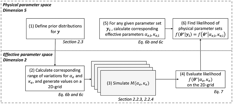
Figure 2. Calculation of the likelihood function with the dimensionality reduction. The computational burden resides in the computation of model outputs M in step 3. Computing model outputs in the effective parameter space reduces the computational burden by going from a parameter space with dimension 5 [O(N5) simulations] to 2 [O(N2) simulations].
Note that in this approach, the two-dimensional effective parameter space is used as a way to reduce the number of forward model simulations needed to evaluate the five-dimensional likelihood function. Once the likelihood is assessed in the five-dimensional space with the procedure described above, the posterior can be calculating by multiplying with the prior pdf (Equation 1). Prior and posterior pdfs remain always defined as a function of the five-dimensional physical parameters.
2.2.3. Analytical Solution
Under specific conditions, there exists an analytical solution to the heat equation. The solution was first introduced by Stallman (1965) and has been widely applied for estimating water exchanges between streams and aquifers from vertically-distributed temperature time series (e.g., Goto et al., 2005; Hatch et al., 2006; Kalbus et al., 2006; Luce et al., 2013). It models the propagation of diurnal temperature fluctuations with depth under the following conditions: the stream temperature is strictly sinusoidal with amplitude θamp, mean θμ, and period P, the HZ temperature at infinite depth is constant in time and equal to the mean of the stream temperature, the hydraulic head difference ΔH between the stream and the bottom of the hyporheic zone column is constant in time. Under these assumptions, the solution to the heat equation is:
where (αe, κe) are calculated from physical properties y (Equations 6b and 6c).
In this study, we leverage this analytical solution as a synthetic study to investigate the identifiability of HZ properties under multiple physical configurations. Numerical values used in this synthetic study are summarized in Table 3. The thermal amplitude of 1°C corresponds to the average in situ diurnal amplitude measured with the LOMOS-mini in the field. For a given set of properties y and hydraulic head difference , outputs of the process-based model M(y) are temperatures at depths −0.1, −0.2, and −0.3 m below the surface obtained with the analytical solution (Equation 8).
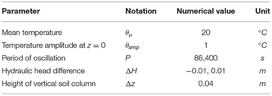
Table 3. Numerical values for variables in analytical solution.
Synthetic observations θ* are obtained by adding a Gaussian white noise to the analytical solution with standard deviation σ = 0.01°C, reproducing the error that was characterized in the lab for temperature sensors used in the field (Cucchi et al., 2018).
2.2.4. Numerical Solution
Temperature and pressure boundary conditions encountered in the field often didn't follow the hypotheses behind the analytical solution described in the previous section. Therefore, for field case study datasets, we solved the physical model described in section 2.2.1 using a numerical solution. The numerical model used is called Ginette (Rivière et al., 2014, 2019) and is available on the GitHub repository https://github.com/agnes-riviere/ginette. It solves the flow and heat transport in saturated sediments using the finite volumes numerical scheme. We use a grid discretization of 1 cm and an adaptive time stepping ensuring convergence of numerical simulations. The hydraulic head difference measured by the LOMOS-mini device is used to define the hydraulic head boundary condition of the model, the top and bottom measured temperature time series are used as top and bottom temperature boundary conditions. The thickness of the model is set to distance between the top and the bottom probes as implemented during the field campaigns, here 40 cm. Since the initial pressure and temperature conditions within the HZ column are unknown, we set up the initial temperature and pressure fields as linear interpolations of pressure and temperature measurements in order to start with realistic initial values, and introduce a burnout time of 4 days that is not further considered in the inversion (Cucchi et al., 2018). The Bayesian inversion is carried out using the remainder of the LOMOS-mini records. Outputs of the process-based model M(y) are temperatures calculated with this numerical model and at depths corresponding to locations of the LOMOS-mini temperature probes.
In this study, the computation time of the numerical model for one given set of parameters converged from about 10 s to more than 15 min, depending on parameter values. For each field dataset, the numerical model was run 10,000 times. Simulations were carried out using parallel computing thanks to computing resources at the National Energy Research Scientific Computing Center (NERSC).
In this paper, process-based forward model refers either to the analytical solution, or to the numerical model.
2.3. Definition of the Prior pdf
The prior pdf fY(y) represents the knowledge about the target parameters Y before accounting for data measured in situ. Two approaches can be adopted when defining a prior pdf (e.g., Gelman et al., 2014). The first approach consists in starting from a case of ignorance, where minimal information is included about the parameter (e.g., equal probabilities between physically-plausible values); in that case the prior is said to be non-informative. The second approach consists in providing a non-trivial amount of information about the target variable, either assumed or collected from other geologically similar sites (e.g., Li et al., 2018; Cucchi et al., 2019). The prior then summarizes previous experience working with variables y; in that case the prior is said to be informative.
In this study, both approaches are adopted sequentially. The purpose of section 3 is to show to what extent the presented measurement strategy allows the estimation of subsurface properties and exchanged fluxes, the prior pdf is hence defined as non-informative uniform between physically realistic bounds (as defined in Table 2). The purpose of section 4 is to estimate HZ properties in the previously studied Avenelles basin where previous work has already helped characterize streambed materials (Mouhri et al., 2013), hence priors there are defined as informative. Estimates resulting from the use of non-informative priors are also computed for comparison purposes.
2.4. Estimation of HZ Physical Properties and Water Fluxes
Applying Bayes' theorem (Equation 1) with prior distributions as defined in section 2.3 and the likelihood function as defined in section 2.2.2 yields the posterior pdf for the physical unknown HZ properties Y = (n, ρs, cs, λs, k), . This posterior pdf is a joint pdf and expresses the probability of any given set of these 5 parameters.
To evaluate the identifiability of a given physical property, say intrinsic permeability k, we compare its prior distribution fK(k) to its posterior distribution (section 2.1). We therefore need to calculate its posterior distribution without the reference to the other unknown HZ properties in Y, where Y = (n, ρs, cs, λs, k). In statistical terms, this is done by calculating the marginal distribution of k from the joint distribution .
For each physical property, the 95% credible interval is also calculated, it is defined such that the posterior probability that the parameter is in the credible interval is 0.95 (Wasserman, 2004).
Finally, the posterior distribution for the specified discharge q is estimated applying Darcy's law (Equation 4) where the intrinsic permeability k is characterized by its posterior distribution (Equation 9).
2.5. Characterizing the Thermal Regime With the Peclet Number
The adimensional Peclet number (Pe) quantifies the ratio of advective to conductive heat fluxes and characterizes the thermal regime of a system (Anderson, 2005). Many formulations of the Peclet number exist (van der Kamp and Bachu, 1989), it has been applied to surface-subsurface exchanges and necessitates the definition of a characteristic length for the physical system under study (e.g., Munz et al., 2011; Bhaskar et al., 2012). Although the characteristic length for the Peclet number is often defined as a function of grain size (e.g., Bhaskar et al., 2012), here we applied dimensional analysis from the heat transport equation (Equation 6a) and calculated the definition of Pe by taking the ratio of the advective to conductive terms in the equation (e.g., Kundu et al., 2012). This yields:
where ΔH [m] is the hydraulic head difference between the stream and the bottom of the hyporheic zone column. For the range of property values used in this study (Table 2), the Peclet number varied between 10−4 and 104.
In this study, we use the Peclet number to characterize the hydrothermal regime of water and heat exchanges in the HZ and to investigate the associated identifiability of hydrological and thermal HZ properties.
3. Estimation of HZ Properties and Fluxes: Synthetic Case Study
We first assess the proposed approach on synthetic cases via the analytical solution to the water and heat transport in the streambed (section 2.2.3). As detailed in Table 4, we focus on six configurations covering a range of HZ water and heat regimes, combining advective, transition and conductive cases, as well as infiltrating and exfiltrating conditions. The definition of the six configurations allows to investigate hydrogeological controls of parameter identifiability. For each configuration, we calculate the likelihood function for the effective parameters (Equation 7), and the corresponding posterior distributions of HZ physical properties (Equation 9). The last subsection generalizes the study to a wide variety of configurations covering the range of variability of physical parameters, as defined in Table 2, for evaluating identifiability of the specific discharge q.
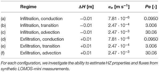
Table 4. Hydrological and thermal configurations in synthetic case study.
3.1. Likelihood of Effective Parameters
Figure 3 shows the likelihood function as a function of effective parameters (Equation 7), for each configuration defined in Table 4. Underlying “true” parameters αe and κe, used to generate the synthetic observed temperature time series θ*, are represented with a wide dot. The thick solid line represents the set of parameters corresponding to Pe = 1, that is the separation between HZ properties corresponding to a conductive regime (left of the line) and properties corresponding to an advective regime (right of the line).
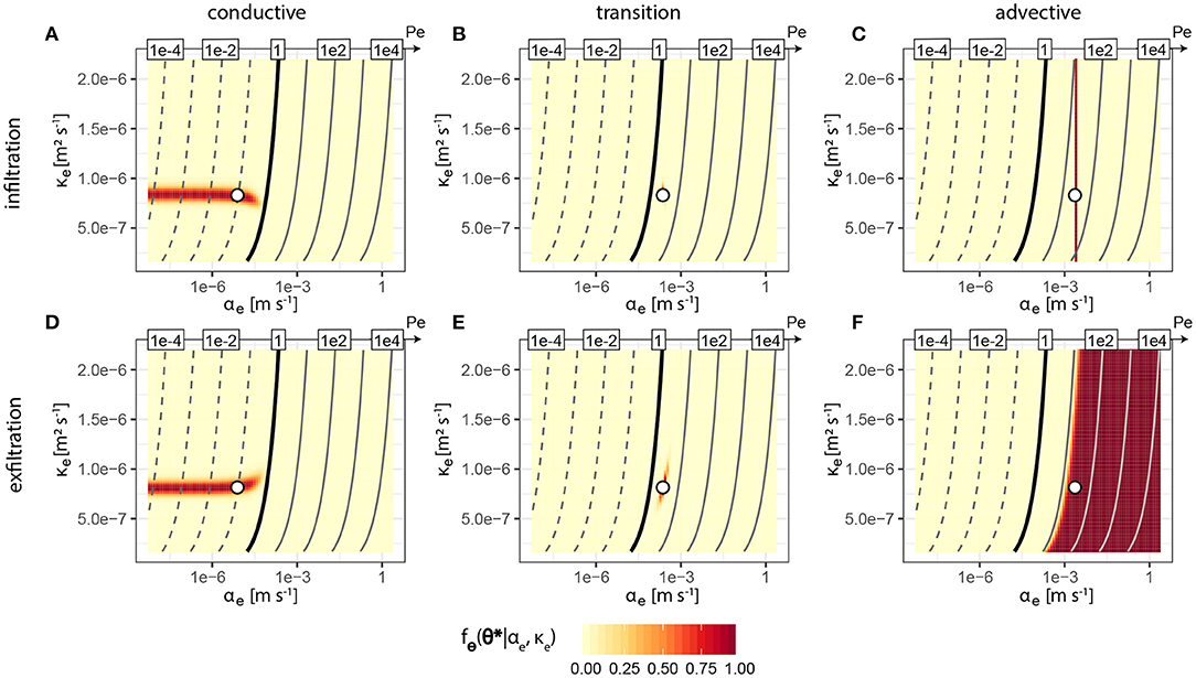
Figure 3. Likelihood values as a function of advective effective parameter αe and conductive effective parameter κe (Equation 7), calculated from synthetic observed time series θ* (section 2.2.3). Panels a-f refer to the hydrological and thermal regimes as defined in Table 4. In each figure, values are normalized from 0 to 1 so that the same color scale can be applied, the x-axis is on a log-scale. The white dot represents the true parameters used to generate θ*. The contour lines signify constant values of Peclet number (thick black: Pe = 1, dashed gray: Pe < 1, solid gray: Pe > 1, one line per unit on the decimal logarithmic scale).
For all configurations, the underlying “true' parameters are located in a region of high likelihood—in other words, the Bayesian inference correctly predicted that the “true” parameters are likely based on the measured data. However, the identifiability of each parameter varies amongst the different combinations, where in some cases (e.g., Figure 3F) the region of high likelihood covers a wide range of αe and κe values leading to low identifiability, whereas in other cases (e.g., Figure 3E) the region of high likelihood is located in a small range of αe and κe, leading to high identifiability.
Effective parameters are best identifiable at the transition between advective and conductive cases under infiltrating and exfiltrating cases (Figures 3B,E). Indeed, for these configurations, the likelihood function peaks around the true parameters values, and is close to zero outside of the underlying parameter combination.
Under conductive conditions for both infiltrating and exfiltrating cases (Figures 3A,D), κe is well-identified, as the high likelihood region is contained within a narrow interval of the effective conductive parameter κe. However, αe is not identifiable, as the high likelihood region extends over a wide interval of αe. However, the high likelihood region for αe is bounded by a maximum value, as the high likelihood region is contained within the conductive region corresponding to Pe < 0.5. This result can be explained physically : under conductive conditions, the conductive term (a function of κe) dominates over the advective term (a function of αe) in the heat equation (Equation 6a). Therefore temperature measurements are sensitive to the value of κe and insensitive to the value of αe—as long as it is small enough for the advective term to remain small when compared to the conductive term. As a result, the likelihood region covers a narrow range for κe and a wide range for αe.
Under advective conditions, the effective conductive parameter κe is never identifiable, as the region of high likelihood covers the entire range of variation of κe (Figures 3C,F). Under advective and infiltrating conditions (Figure 3C), the effective advective parameter αe is identified to be in a narrow interval, whereas under advective exfiltrating conditions (Figure 3F), the effective advective parameter αe is bounded to a region corresponding to Pe > 5. This result can again be explained physically : under advective conditions, the advective term (a function of αe) dominates over the conductive term (a function of κe) in the heat equation (Equation 6a), temperature measurements are sensitive to the value of αe and insensitive to the value of κe. As a result, the likelihood region covers a narrow range for αe and a wide range for κe. Additionally, under infiltrating conditions, the infiltrating water propagates the diurnal temperature signal with depth, and this propagation is a function of the advective parameter value αe. In contrast, under exfiltrating conditions, the diurnal temperature variations do not propagate with depth, and the observed temperature time series is constant. Therefore, under highly advective conditions (Pe > 5), parameter αe is identifiable within a narrow range under infiltrating conditions, while the uncertainty is higher under exfiltrating conditions.
In summary, the effective advective parameter αe is identifiable at least to be within a region for all configurations, as for all configurations an upper or lower bound exists. A clear cut exists between the advective regime (Pe > 5) and the conductive regime (Pe < 0.5), where regions of likely values do not cross the middle domain (0.5 < Pe < 5). As αe varies over a much larger range than κe, the value of αe has a strong influence on the value of the Peclet number and dominates the physical behavior of the soil column and the corresponding time series produced by the model.
3.2. Posterior Intrinsic Permeability Distribution
Figure 4 shows prior and posterior distributions for intrinsic permeability for the six investigated flow and heat regimes, as well as the associated underlying “true” permeability value and the posterior credible interval. For all regimes, the posterior distributions are narrower than the priors and the true value for the intrinsic permeability is located within the credible interval, which confirms that the algorithm correctly infers the interval where intrinsic permeability is located based on the observed temperature time series.
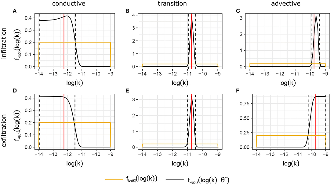
Figure 4. Prior (in yellow) and posterior (in black) distributions for log-transformed permeability. Panels a-f refer to the hydrological and thermal regimes as defined in Table 4. The vertical red bars are values of underlying parameters used to generate synthetic measurements θ*. The dashed black lines represent the bounds of the 95% credible intervals. For all regimes, the underlying value for the intrinsic permeability is located within the credible interval, which confirms that the algorithm correctly infers the interval where intrinsic permeability is located based on the observed temperature time series. Posterior distributions are always narrower than priors, showing that temperature time series are always helpful for characterizing intrinsic permeability values. The posterior distributions are narrower for transition and advection cases, for conductive cases intrinsic permeability values are characterized to be lower than the upper bound ~ 10−12m2, i.e., a hydraulic conductivity value of ~ 10−5m · s−1.
However, the width of the credible interval is variable between the regimes (Figure 4). In the advective and transition cases, the intrinsic permeability is identified to be in a narrow region around the true value. In the conductive case, it is identified to be bounded by a maximum value. The local peak in the infiltrating case confirms that if the posterior distribution remains wide, highest likelihood values are identified to be located around the true underlying intrinsic permeability value—and that intrinsic permeability is better identified in infiltration cases where temperature variations at the surface penetrate deeper in the streambed (Figure 4A). These findings are in line with the identifiability of effective parameter αe described in the previous section, as intrinsic permeability k represents most of the variability of the effective advective parameter αe (Equation 6c). In the conductive regime, heat transport is dominated by conduction and thus mostly insensitive to flow which is mostly controlled by permeability values, while in the advective and transition regime heat transport is sensitive to the advective term which is directly proportional to intrinsic permeability.
Posteriors for intrinsic permeability k are more certain (less wide) than posteriors for physical parameters n, λs, cs, and ρs, for which the posterior credible intervals cover almost the total variation range of the variation defined by prior distributions (not shown here). This is because these 4 parameters vary within similar orders of magnitude, such that a unique value of κe can correspond to many combinations of n, λs, cs, and ρs. As a result, even in cases when κe is known to be within a narrow interval, each of these parameters can still cover a wide range of values. These parameters cannot be individually estimated from vertically-distributed temperature alone.
3.3. Estimation of Specific Discharge
In this section, we investigated the inference of specific discharge based on vertically-distributed temperature measurements for HZ properties covering the variation range (Table 2). For the investigated parameter sets, the “true” specific discharge values q range between q = −10−4 m s−1 (−8 m d−1, infiltration) and q = 10−4 m s−1 (8 m d−1, exfiltration). The predicted specific discharge q from measured temperatures is calculated following equation 10. Figure 5 shows the 95% credible interval of each estimated specific discharge as a function of the “true” specific discharge value, where the 1:1 line represents perfect prediction.
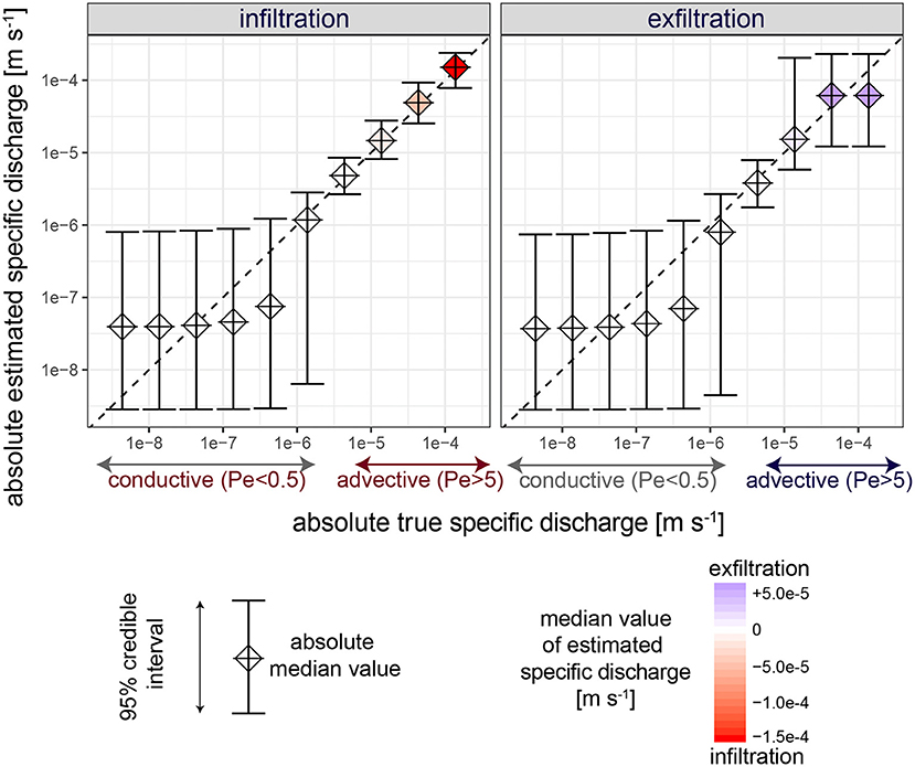
Figure 5. Statistics of estimated specific discharge: median and 95% posterior credible intervals, Pe ∈ [0.01, 100]. Axes are on the logarithmic scale. Specific discharge is identifiable above 2 · 10−6 m s−1 (17 cm d−1), where the width of the 95% posterior credible interval ranges over half an order of magnitude.
3.3.1. Specific Discharge Estimates for Pe>0.5
Estimates of absolute specific discharge ranging between 2 · 10−6 m s−1 (17 cm d−1) and 10−4 m s−1 (8 m d−1) match true specific discharge values with good confidence (Figure 5). Indeed, for those high specific discharge values discharging into or out of the HZ, the width of the 95% posterior credible interval only ranges over half an order of magnitude. This configuration corresponds to either an advective (Pe>5) or a transitional (0.5<Pe<5) hydrothermal functioning of the HZ.
3.3.2. Conductive Functioning (Pe<0.5)
Estimates of specific discharge for low specific discharge values (|q| < 10−6m s−1, i.e., (8 cm d−1) are characterized by more uncertainty. These cases correspond to a conductive functioning of the HZ, for which the intrinsic permeability posterior pdf is only known to be bounded by an upper value (Figure 4A). Therefore, the posterior credible interval for specific discharge is similar for all conductive cases, with a median value of 4 10−8 m s−1, i.e., 3.5 mm d−1. In these cases, estimates of the specific discharge are uncertain, ranging over two orders of magnitude.
3.3.3. Infiltration vs. Exfiltration for Pe>50
In a highly advective configuration (Pe>50), uncertainty is smaller under infitrating configurations than under exfiltrating configurations. Indeed, under high values of exfiltrating specific discharge, HZ temperatures are governed by groundwater temperatures which are stable in time. In that case, diurnal temperature variations of the stream do not penetrate with depth in the HZ, and specific discharge values can only be estimated to be higher than a critical specific discharge value defining the highly advective case. On the contrary, under high infiltrating conditions, high specific discharges propagate diurnal temperature variations down the HZ, and specific discharges are estimated to be within a narrow posterior credible interval. Our examples are based on a 1°C amplitude in the stream, which is the low bound of temperature time series amplitudes measured in the field, it is worth noting that the uncertainty could be decreased with higher stream temperature amplitudes.
In conclusion, the synthetic case study showed that identifiability depends on the Peclet number. When 0.5<Pe<5, both advective and conductive parameters are identifiable with narrow posterior pdfs, while in conductive (Pe<0.5) or advective (Pe>5) conditions, only associated properties are identifiable.
4. Estimation of HZ Properties and Fluxes: Field Case Study
This section presents the application of the methodological framework to time series collected in the Avenelles basin, France. The Avenelles sedimentary basin is located 70 km East of Paris and mainly used for agriculture (Loumagne and Tallec, 2013). In this well-instrumented experimental basin, a monitoring network has been designed and implemented in order to quantify stream-aquifer exchanges over multiple spatial and temporal scales. LOMOS-mini devices are installed in this basin in order to complement this monitoring network in place (Mouhri et al., 2013). The streambed is composed of loess and underlaid by colluvium with blocks of gritstone, a rarely sampled type of hyporheic zone.
4.1. In situ HZ Monitoring
HZ properties estimation is based on in situ measurements obtained using the LOMOS-mini monitoring device—its functioning is briefly summarized here, for more information we refer the reader to Cucchi et al. (2018). The LOMOS-mini consists in the coupling of temperature and pressure measurements (Figure 1). Several temperature sensors are vertically distributed. One is located in the stream and four are located at multiple depths below the streambed, where the deepest temperature sensor is placed between 40 and 60 cm below the streambed. In the direct vicinity of the temperature sensors, a piezoresistive pressure sensor is hydraulically connected to two tubes, one in the river and one in the HZ. It records the hydraulic head difference between the stream and the HZ at depth. All temperature and pressure measurements are synchronous and recorded with a 15 min-periodicity and for a duration of 1–3 weeks. Figure 6 presents two examples of measured data sets in the Avenelles basin.
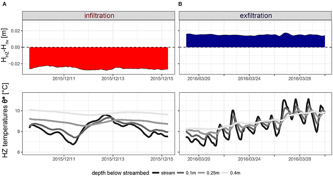
Figure 6. LOMOS-mini measurement data sets used to estimate hydrothermal properties and fluxes. Top row: pressure head difference ΔH. Bottom row: HZ 1D vertically-distributed temperatures. Two configurations are presented: (A) infiltration case study and (B) exfiltration case study.
4.2. Likelihood of Effective Parameters
The inversion framework was applied to the 2 sets of LOMOS-mini measurements presented in Figure 6 in order to derive uncertainty-quantified estimates of HZ properties and fluxes in the streambed. For the field case study, the inversion was carried out using the numerical model described in section 2.2.4.
Figure 7 presents the corresponding likelihood function corresponding to measurements as a function of effective parameters. Root mean squared errors between measured time series and time series simulated for parameters with the highest likelihood are 0.065°C for the infiltrating point and 0.043°C for the exfiltrating point, suggesting that the modeling approach was able to reproduce the observed temperature values.
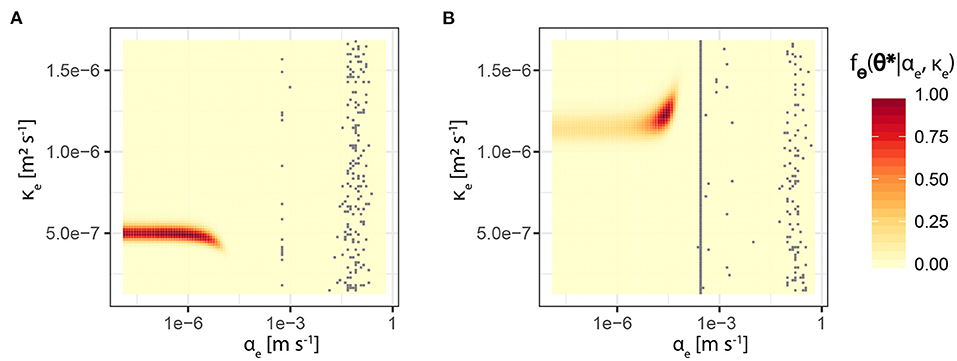
Figure 7. Normalized likelihood functions as a function of advective effective parameter αe and conductive effective parameter κe, (A,B) refer to the two LOMOS-mini measurement datasets presented in Figure 6, corresponding to an infiltration and an exfiltration case study respectively. In each panel, values are normalized so that the same color scale can be applied, the x-axis is plotted on a log-scale. For grayed-out combinations of αe and κe, numerical simulations have not converged within the allocated time (15 min) and no likelihood value can be computed. By comparing with the analytical study results (Figure 3), point (A) seems to undergo a conductive regime where high likelihoods are restricted within a narrow interval of κe and high likelihood are bounded by a maximum value for αe, while point (B) seems to undergo a transition regime where both κe and αe can be well-characterized from LOMOS-mini measurements.
Figure 7 can be interpreted in the light of results of the analytical case study, in particular by comparison with likelihood functions derived for infiltrating or exfiltrating boundary conditions, and advective or conductive thermal regimes (Figure 3). Point a corresponds to infiltrating boundary conditions in a conductive thermal regime (Figure 3A). In that case, the effective conductive parameter κe is identifiable to be located in a narrow interval, and the effective advective parameter αe is identified to be bounded by a maximum value corresponding to the transition from a conductive to an advective thermal regime. Point b corresponds to the configuration where hydrological boundary conditions are exfiltrating and the thermal regime is at the transition between advective and conductive conditions (Figure 3E). In that case, both effective parameters αe and κe are identifiable.
4.3. Identification of Physical Properties
We then investigate posterior distributions of two physical subsurface properties: the intrinsic permeability k and the thermal conductivity λs. Here, two scenarios for defining prior distributions were tested. The first scenario is in line with the synthetic study in section 3, where priors were defined as uniform bounded between physically reasonable values, as defined in Table 2. The second scenario corresponds to a case where the prior stay non-informative for parameters corresponding to permeability k and thermal conductivity λs, but we assume that porosity n, sediment density ρs and sediment heat capacity cs to be informative, where associated prior distributions are defined as uniform distributions within narrower intervals: n ∈ [0.2, 0.3], ρs ∈ [2000, 2300] kg m−3, and cs ∈ [1000, 1500] m2 s−2 C−1. Figure 8 shows associated posterior distributions, where posteriors associated with the first scenario are represented in black and ones with the second scenario in gray.
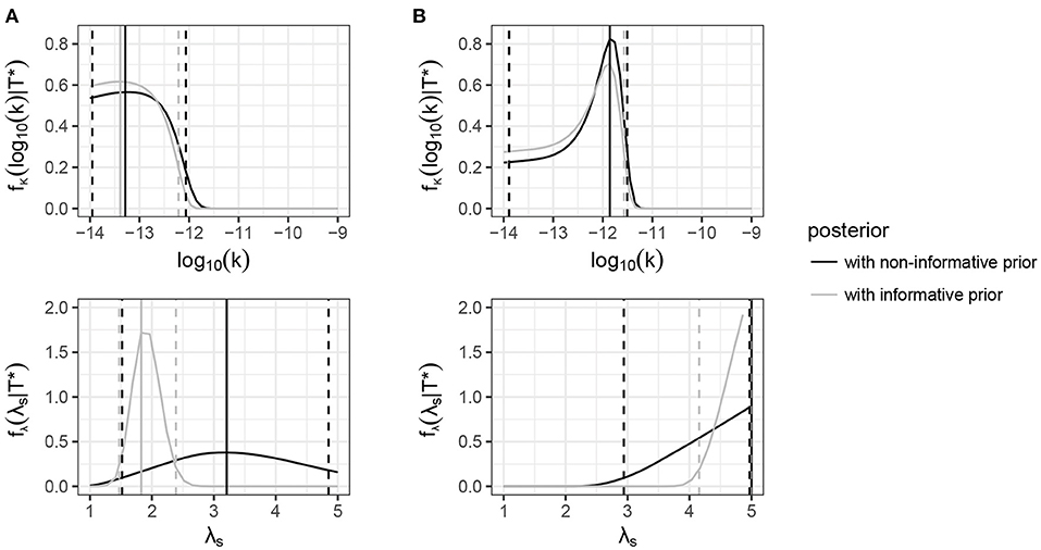
Figure 8. Posterior pdfs for intrinsic permeability k and heat conductivity λs at both investigated locations, marginalized from the multivariate posterior distributions. Panels (A,B) refer to the two LOMOS-mini measurement datasets presented in Figure 6, corresponding to an infiltration and an exfiltration case study respectively. The black lines represent the posterior derived from non-informative priors and the gray lines represent the posterior derived from informative priors. The solid vertical lines represent the maximum a posteriori estimate and the dashed vertical lines represent the 95% posterior credible interval.
4.3.1. Posterior of Intrinsic Permeability
For point a, the maximum a posteriori estimate for intrinsic permeability is k = 5.2 · 10−14 m2, and the 95% posterior credible interval is [1.1 · 10−14, 8.6 · 10−13] m2. The intrinsic permeability is identified to be bounded by a maximum value, in line with the observation that the effective advective parameter αe is bounded by an upper value. For point b, the maximum a posteriori estimate for intrinsic permeability is k = 1.4 · 10−12 m2, and the 95% posterior credible interval is [1.29 · 10−14, 3.1 · 10−12] m2. Again, the intrinsic permeability is identified to be bounded by a maximum value. These local posterior distributions constitute the final result for the estimation of hydrological and thermal properties from LOMOS-mini measurement sets.
4.3.2. Posterior of Thermal Conductivity
For point a, the maximum a posteriori estimate for thermal conductivity λs is λs = 3.2 W m−1 K−1, and the 95% posterior credible interval is [1.5, 4.8] W m−1 K−1. For point b, the maximum a posteriori estimate for thermal conductivity λs is λs = 5 W m−1 K−1, and the 95% posterior credible interval is [2.9, 5] W m−1 K−1. It is interesting to note that posterior pdfs for λs are wide even if the likelihood functions for the conductive effective parameter κe are located within a narrow range of variation (Figure 7). This is because κe is a function of λs, n, ρs and cs, and the ranges of variation of properties n, ρs and cs are comparable to the range of variation of λs (Equation 6b). Therefore, uncertainty in parameters n, ρs and cs lead to uncertainty in λs estimates even if κe is well-identified.
4.3.3. Informative Prior Distributions
Using informative prior distributions for n, ρs and cs results in narrower posterior distributions in λs, while estimates of permeability k are almost unchanged with the use of informative prior distributions (Figure 8). This is because the variation range of parameters other than k is small when compared to the variation range of k. It appears that LOMOS-mini measurements alone allow for the identification of intrinsic permeability without the need for informative priors for n, ρs, and cs.
4.4. Estimation of Specific Discharge
The posterior predictive distribution for the time series of specific discharge can be calculated by applying Darcy's law (Equation 4) using the posterior pdf of intrinsic permeability (Figure 8). 100 values of intrinsic permeability k were sampled from the posterior pdf, and for each permeability sample, a time series of specific discharge was simulated using the forward numerical model, yielding an ensemble of exchanged time series realizations. From this ensemble, values corresponding to the 2.5th, 25th, 50th, 75th, and 97.5th percentiles were extracted.
At point a, the median value of the specific discharge is estimated to be around 5 · 10−8 m s−1 (0.4 cm d−1), ranging between 1 · 10−8 and 5 · 10−7 m s−1 with 95% uncertainty (Figure 9A). At point b, the median value of the specific discharge is estimated to be around 2 · 10−7 m s−1 (1.7 cm d−1), ranging between 5 · 10−9 and 1 · 10−6 m s−1 with 95% uncertainty (Figure 9B).
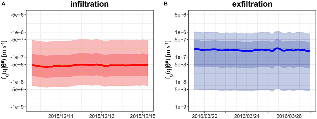
Figure 9. Posterior distributions of specific discharge q. Panels (A,B) refer to the two LOMOS-mini measurement datasets presented in Figure 6, corresponding to an infiltration and an exfiltration case study respectively. The solid lines represent the medians of the posterior distributions, the shaded intervals correspond to the 50 and 95% posterior intervals. The y-axis is on a logarithmic scale.
5. Discussion
This paper introduced a solution combining field instrumentation, process-based numerical modeling, and Bayesian inference to estimate hydrothermal properties and high-frequency water and heat fluxes in the HZ. This solution relies on measurements from the LOMOS-mini, a sensor that is cost-effective (< 500 euros), easy to manipulate, and quick and robust to deploy on the field (Cucchi et al., 2018). This solution complements the set of available solutions for estimating surface-subsurface exchanges (see Kalbus et al., 2006 and Ren et al., 2018 for comprehensive reviews).
Uncertainty is common to subsurface data due to data scarcity and subsurface variability, and quantifying and accounting for uncertainty is recognized as fundamental for decision making in hydrogeology (e.g., Gelhar, 1993; Rubin, 2003; Kitanidis, 2015). As opposed to deterministic approaches typically adopted in previous HZ studies, the stochastic point of view adopted in this study invoked probability concepts to deal with problems of physics, where unknown properties are modeled as random variables characterized by their probability distributions. Amongst methods adopting the stochastic point of view, the Bayesian inference presented in section 2—in which probabilities are updated as more information or measurements become available—has been used in a wide range of settings in hydrological and hydrogeological studies (e.g., Woodbury, 2007; Freni and Mannina, 2010; Rubin et al., 2010; Harrison et al., 2012; Viglione et al., 2013; Zhang et al., 2014; Linde et al., 2017). Bayesian inference is flexible in the amount of information to account for prior to starting the assimilation of in situ measurements (Rojas et al., 2009; Kitanidis, 2012; Cucchi et al., 2019; Heße et al., 2021). To the author's knowledge, this study is the first to adopt a stochastic or Bayesian approach for estimating properties and fluxes from measurements in the HZ and it demonstrated how estimates become more reliable as the amount of prior information increases.
Here, the Bayesian framework allowed to investigate how LOMOS-mini measurements could support the estimation of unknown HZ properties (i.e., hydraulic conductivity, porosity, thermal conductivity, thermal capacity, density). We have proposed a new formulation for the Peclet number in the framework of surface-subsurface water exchange quantification using LOMOS-mini measurements (Equation 11) and demonstrated the strong relationship between this Peclet and estimates of HZ properties, where regions of likely values do not cross the domain around Pe = 1. We showed that LOMOS-mini measurements allowed to estimate hydraulic conductivity within less than one order of magnitude for hydraulic conductivities greater than ~10−5m · s−1 even when all other properties are unknown, and that this uncertainty decreases when other properties are better characterized prior to starting the measurement assimilation procedure. Previous studies demonstrated how uncertain HZ properties result in incorrect discharge calculations (e.g., Shanafield et al., 2011), with the Bayesian framework presented in this study, uncertainties in HZ properties are accounted for on flux estimates in a way that is transparent and coherent. Another application of such framework is goal-oriented campaign design, where field campaigns are optimized so that they maximize the expected data worth (e.g., Nowak et al., 2012; Harken et al., 2019). For example, if the goal of a given campaign is to estimate hydraulic conductivity, one should favor field measurements collected in high-flow conditions (e.g., winter) over low-flow conditions.
Previous studies have relied on vertically-distributed temperature measurements such as ones collected by the LOMOS-mini to estimate HZ properties. A sentinel study from Lapham (1989) demonstrated the feasibility of determining hydraulic conductivities from streambed temperature time series, they assumed known values for unknown parameters density and thermal diffusivity and used a numerical model to represent water and heat transport. More recently, Hatch et al. (2010) used a combination of automated vertically-distributed temperature measurements and manual hydraulic gradient measurements to estimate hydraulic conductivity. They assumed known values for porosity, fluid and sediment density and heat capacity, and thermal dispersivity in the streambed, as well as steady state conditions for each calculation of a daily mean water flux value. While their approach allows for easiness of data handling, the obtained fluxes and HZ properties values do not account for uncertainty in HZ properties estimates, and do not apply for estimating dynamic (sub-daily) seepage rates. Other studies have used vertically-distributed temperature time series to estimate hydraulic conductivity and seepage (e.g., Niswonger and Prudic, 2003; Stoneman and Constantz, 2003; Burow et al., 2005) or HZ properties relating to thermal transport (e.g., Luce et al., 2013; Vandersteen et al., 2015), but our method is the first to jointly estimate all unknown HZ properties (i.e., hydraulic conductivity, porosity, thermal conductivity, thermal capacity, density) as well as vertical discharge values. A fundamental assumption of such approaches, including the one developed in this paper, is that flow and heat transport locally occur along a one-dimensional vertical direction. Although relevant in most cases given the spatial distortion between the longitudinal dimension (decameter) and the vertical one (centimeter) (Flipo et al., 2014), the local one-dimensional assumption can lead to errors in specific discharge estimates in cases of low specific discharge and highly heterogeneous streambeds (e.g., Salehin et al., 2004; Ferguson and Bense, 2007; Irvine et al., 2012, 2015a; Cuthbert and MacKay, 2013).
Recently, Thomle et al. (2020) introduced a new probe for quantifying dynamic exchange at the interface between surface water and groundwater via the monitoring of temperature, pressure, as well as electrical conductivity along a vertical profile. This probe is very similar in design to the LOMOS-mini sensor used in this study, the main difference being the presence of electrical conductivity measurements. They showed that adding pressure head difference measurements to temperature profiles lead to accurate estimates of porosity and permeability. Although having developed one of the most advanced electrogeophysical probe for HZ applications, the testing of this probe was performed in a controlled soil column and this probe has not been deployed in in situ conditions yet. The price of the probe in Thomle et al. (2020) was not mentioned, however the LOMOS-mini would be a more cost-effective choice (since it doesn't require electrical conductivity measurements) in cases when vertical pore water velocity estimates are not needed. Finally, the Bayesian measurement assimilation framework introduced in this study could also be applied to measurements collected with the probe designed in Thomle et al. (2020), leading to uncertainty-quantified estimates of in situ water and energy fluxes under transient conditions with a temporal resolution of a few minutes, as well as associated uncertainty-quantified HZ properties.
While it is well-established today that high-frequency datasets are required to fully capture the biogeochemical functioning of river and streams systems, the hyporheic datasets remain coarse as regards to time sampling (Aubert et al., 2015; Vilmin et al., 2016; Floury et al., 2017; Escoffier et al., 2018; Wang et al., 2019). Rapid hydrological events such as storms can be key drivers of increased exchange between stream water and groundwater in the HZ, thereby fueling HZ nitrate reduction processes and modifying the large-scale biogeochemical function of the HZ (e.g., Dudley-Southern and Binley, 2015). Providing high frequency flow is key to better understand the role played by the stream-aquifer interface in the functioning of the critical zone, particularly for small stream orders where stream ecology is mostly controlled by benthic processes (Flipo et al., 2004, 2007; Gaillardet et al., 2018; Jäger and Borchardt, 2018; Segatto et al., 2020). How and how much HZ processes contribute to river ecology in average or at very short time scale is still an open research question. For instance, Newcomer et al. (2018) demonstrated that flow direction control carbon emission to rivers by bacterial respiration in the HZ, thereby suggesting that high-frequency measurements are required to assess carbon emissions by rivers toward the atmosphere. The LOMOS-mini system and the assimilation technique proposed in this paper overcome the temporal sampling limitation and provide a unique tool for further investigating the hydrological and biogeochemical role played by the HZ at the catchment scale.
The monitoring and data assimilation methodology introduced in this study can further contribute to innovative research focused on measurement of HZ fluxes. Indeed, drivers of HZ exchanges are complex, they include topographically-varying bedforms such as ripples or pool-riffle sequences, river sinusoity, changes in hydraulic conductivity of sediments, high-frequency pressure variations resulting from rainfall events and low-frequency pressure variations resulting from flows in regional aquifer systems (Elliott and Brooks, 1997; Malard et al., 2002; Cardenas et al., 2004; Fleckenstein et al., 2006; Cardenas and Wilson, 2007; Flipo et al., 2014). The quantification of fluxes between streams and aquifers remains challenging and their impact on environmental and water management remains often underestimated due to a lack of experience for measurement and analysis approaches (Lewandowski et al., 2020). One relatively recent and promising direction is the development of Fiber-Optic Distributed Temperature Sampling (FO-DTS). FO-DTS can identify areas of groundwater discharge continuously along the streambed—often with mixing models that only consider the advective component of heat transfers (Selker et al., 2006a; Briggs et al., 2012). Simon et al. (2021) demonstrated with laboratory experiments the accuracy of discharge flux estimates offered by the combination of a heat source with a FO-DTS over a range spanning 1 10−6 to 5 10−2 m s−1. The methodology introduced in this study can not only serve as an in situ validation system for these innovative measurements, but also complement experimental set-ups for high-frequency discharge flux estimation, in particular at hot spot locations (Zhao et al., 2021). FO-DTS systems have recently been coupled with vertically distributed temperature sensors for quantifying water exchanges along the FO (Shanafield et al., 2018; Le Lay et al., 2019). Since our methodology allows to lift the classical assumption of a daily hydraulic steady state, coupling FO-DTS with LOMOS-mini monitoring systems would open the door to the interpretation of FO-DTS datasets collected outside of low-flow steady-state events. This would provide unique datasets for characterizing not only HZ properties, but also HZ water and energy fluxes both continuously along the stream and during transient high-flow events, such as floods or flow reversal following a rainfall event.
6. Conclusion
This study introduced a new solution for estimating HZ properties and surface-subsurface water exchanges, leveraging in situ LOMOS-mini measurements, numerical modeling and Bayesian inference. There are three main innovations in the proposed method. First, Bayesian inference provided a framework for investigating the identifiability of HZ properties from collected measurements, and to derive uncertainty-quantified HZ properties and surface-subsurface water exchange estimates. To the authors' knowledge, this is the first study using Bayesian inference for investigating the HZ. Second, the definition of effective parameters decreased the number of numerical simulations needed and provided a simplified view of the problem, allowing to investigate the identifiability of HZ properties as a function of two parameters summarizing the advective and convective heat fluxes. Third, it introduced a new formulation of the Peclet number describing the hydrological and thermal regime in the HZ and controlling the identifiability of HZ properties; this Peclet number can be calculated from in situ LOMOS-mini measurements.
It demonstrated that the LOMOS-mini is a low-cost and complete stand-alone solution for estimating local stream-aquifer exchanges under dynamic exchange conditions, as well as for quantifying HZ properties with associated uncertainties. The proposed approach complements the set of available solutions for monitoring the HZ, and can contribute to further innovative research into HZ dynamic hydrological and thermal functioning and its role for regulating water availability and quality.
Data Availability Statement
The raw data supporting the conclusions of this article will be made available by the authors upon request, without undue reservation.
Author Contributions
NF and AR conceived the LOMOS-mini monitoring device. KC and YR conceived the Bayesian inversion framework. AR verified the numerical results of the numerical model. KC implemented the Bayesian inversion. KC, AR, and NF carried out field experiments. KC wrote the manuscript with the contribution of AR and NF. YR, NF, and AR reviewed the manuscript. All authors contributed to the verification, interpretation of the results, provided critical feedback, helped shape the research, and analysis the manuscript.
Funding
This research was supported by the Jane Lewis Fellowship from the University of California, Berkeley, the Chateaubriand Fellowship from the French Foreign Affair Ministry, the Department of Civil and Environmental Engineering in University of California, Berkeley, and the Carnot-Mines Traversière. It is a contribution to the PIREN-Seine research program (http://www.piren-seine.fr).
Conflict of Interest
The authors declare that the research was conducted in the absence of any commercial or financial relationships that could be construed as a potential conflict of interest.
Publisher's Note
All claims expressed in this article are solely those of the authors and do not necessarily represent those of their affiliated organizations, or those of the publisher, the editors and the reviewers. Any product that may be evaluated in this article, or claim that may be made by its manufacturer, is not guaranteed or endorsed by the publisher.
Acknowledgments
The authors are grateful to Aurélien Baudin, Asma Berrhouma, Noëlia Carrillo, Nelly Martineau, and Edmée Cuisinier for their contribution to field work. The authors acknowledge the feedback of Prof. Sally Thompson which helped improve the quality of the manuscript. This research used resources of the National Energy Research Scientific Computing Center (NERSC), a U.S. Department of Energy Office of Science User Facility located at Lawrence Berkeley National Laboratory, operated under Contract No. DE-AC02-05CH11231.
References
Anderson, K., and Segall, P. (2013). Bayesian inversion of data from effusive volcanic eruptions using physics-based models: application to Mount St. Helens 2004-2008. J. Geophys. Res. Solid Earth 118, 2017–2037. doi: 10.1002/jgrb.50169
Anderson, M. P. (2005). Heat as a ground water tracer. Groundwater 43, 951–968. doi: 10.1111/j.1745-6584.2005.00052.x
Aubert, A., Mérot, P., and Gascuel, C. (2015). Temporal patterns of water quality: decadal high-frequency data-driven analysis from an hydrological observatory under agricultural land-use. La Houille Blanche Revue internationale de l'eau 6, 5–11. doi: 10.1051/lhb/20150062
Bejan, A. (2013). “Properties of liquids,” in Convection Heat Transfer (Hoboke, NJ: John Wiley & Sons), 625–632. doi: 10.1002/9781118671627.app3
Bencala, K. E. (2000). Hyporheic zone hydrological processes. Hydrol. Process. 14, 2797–2798. doi: 10.1002/1099-1085(20001030)14:15<2797::AID-HYP402>3.0.CO;2-6
Bhaskar, A. S., Harvey, J. W., and Henry, E. J. (2012). Resolving hyporheic and groundwater components of streambed water flux using heat as a tracer. Water Resour. Res. 48, 1–16. doi: 10.1029/2011WR011784
Blasone, R.-S. (2007). Parameter estimation and uncertainty assessment in hydrological modeling (Ph.D. thesis). Technical University of Denmark, Kongens Lyngby, Denmark.
Boano, F., Harvey, J. W., Marion, A., Packman, A., Revelli, R., Ridolfi, L., et al. (2014). Hyporheic flow and transport processes: mechanisms, models, and biogeochemical implications. Rev. Geophys. 52, 603–679. doi: 10.1002/2012RG000417
Boulton, A., Findlay, S., Marmonier, P., Stanley, E. H., and Maurice Vallet, H. (1998). The functional significance of the hyporheic zone in streams and rivers. Annu. Rev. Ecol. Syst. 29, 59–81. doi: 10.1146/annurev.ecolsys.29.1.59
Briggs, M. A., Lautz, L. K., and McKenzie, J. M. (2012). A comparison of fibre-optic distributed temperature sensing to traditional methods of evaluating groundwater inflow to streams. Hydrol. Process. 26, 1277–1290. doi: 10.1002/hyp.8200
Brunke, M., and Gonser, T. (1997). The ecological significance of exchange processes between rivers and groundwater. Freshw. Biol. 37, 1–33. doi: 10.1046/j.1365-2427.1997.00143.x
Brunner, P., Therrien, R., Renard, P., Simmons, C. T., and Hendricks Franssen, H.-J. (2017). Advances in understanding river - groundwater interactions. Rev. Geophys. 55, 818–854. doi: 10.1002/2017RG000556
Burow, K. R., Constantz, J., and Fujii, R. (2005). Heat as a tracer to estimate dissolved organic carbon flux from a restored wetland. Groundwater 43, 545–556. doi: 10.1111/j.1745-6584.2005.0055.x
Cardenas, M. B. (2015). Hyporheic zone hydrologic science: a historical account of its emergence and a prospectus. Water Resour. Res. 51, 3601–3616. doi: 10.1002/2015WR017028
Cardenas, M. B., and Wilson, J. L. (2007). Dunes, turbulent eddies, and interfacial exchange with permeable sediments. Water Resour. Res. 43, 1–16. doi: 10.1029/2006WR005787
Cardenas, M. B., Wilson, J. L., and Zlotnik, V. A. (2004). Impact of heterogeneity, bed forms, and stream curvature on subchannel hyporheic exchange. Water Resour. Res. 40, 1–13. doi: 10.1029/2004WR003008
Carrera, J., and Neuman, S. P. (1986). Estimation of aquifer parameters under transient and steady state conditions: 2. Uniqueness, stability, and solution algorithms. Water Resour. Res. 22, 211–227. doi: 10.1029/WR022i002p00211
Clark, M. P., Bierkens, M. F. P., Samianego, L., Woods, R. A., Uijlenhoet, R., Bennett, K., et al. (2017). The evolution of process-based hydrologic models: historical challenges and the collective quest for physical realism. Hydrol. Earth Syst. Sci. 21, 3427–3440. doi: 10.5194/hess-21-3427-2017
Conant, B. (2004). Delineating and quantifying ground water discharge zones using streambed temperatures. Groundwater 42, 243–257. doi: 10.1111/j.1745-6584.2004.tb02671.x
Constantz, J. (2008). Heat as a tracer to determine streambed water exchanges. Water Resour. Res. 44, 1–20. doi: 10.1029/2008WR006996
Constantz, J., Stewart, A., Niswonger, R., and Sarma, L. (2002). Analysis of temperature profiles for investigating stream losses beneath ephemeral channels. Water Resour. Res. 38, 1–13. doi: 10.1029/2001WR001221
Cosenza, P., Guérin, R., and Tabbagh, A. (2003). Relationship between thermal conductivity and water content of soils using numerical modelling. Eur. J. Soil Sci. 54, 581–588. doi: 10.1046/j.1365-2389.2003.00539.x
Cucchi, K., Heße, F., Kawa, N., Wang, C., and Rubin, Y. (2019). Ex-situ priors: a Bayesian hierarchical framework for defining informative prior distributions in hydrogeology. Adv. Water Resour. 126, 65–78. doi: 10.1016/j.advwatres.2019.02.003
Cucchi, K., Rivière, A., Baudin, A., Berrhouma, A., Durand, V., Rejiba, F., et al. (2018). LOMOS-mini: a coupled system quantifying transient water and heat exchanges in streambeds. J. Hydrol. 561, 1037–1047. doi: 10.1016/j.jhydrol.2017.10.074
Cuthbert, M. O., and MacKay, R. (2013). Impacts of nonuniform flow on estimates of vertical streambed flux. Water Resour. Res. 49, 19–28. doi: 10.1029/2011WR011587
Dudley-Southern, M., and Binley, A. (2015). Temporal responses of groundwater-surface water exchange to successive storm events. Water Resour. Res. 51, 1112–1126. doi: 10.1002/2014WR016623
Elliott, A., and Brooks, N. (1997). Transfer of nonsorbing solutes to a streambed with bed forms: theory. Water Resour. Res. 33, 123–136. doi: 10.1029/96WR02784
Eppelbaum, L., Kutasov, I., and Pilchin, A. (2014). “Thermal properties of rocks and density of fluids,” in Applied Geothermics (Berlin; Heidelberg: Springer-Verlag), 99–149. doi: 10.1007/978-3-642-34023-9_2
Escoffier, N., Bensoussan, N., Vilmin, L., Flipo, N., Rocher, V., David, A., et al. (2018). Estimating ecosystem metabolism from continuous multi-sensor measurements in the Seine River. Environ. Sci. Pollut. Res. 25, 23451–23467. doi: 10.1007/s11356-016-7096-0
Ferguson, G., and Bense, V. (2007). Uncertainty in 1D heat-flow analysis to estimate groundwater discharge to a stream. Groundwater 49, 336–347. doi: 10.1111/j.1745-6584.2010.00735.x
Fleckenstein, J. H., Krause, S., Hannah, D. M., and Boano, F. (2010). Groundwater-surface water interactions: new methods and models to improve understanding of processes and dynamics. Adv. Water Resour. 33, 1291–1295. doi: 10.1016/j.advwatres.2010.09.011
Fleckenstein, J. H., Niswonger, R. G., and Fogg, G. E. (2006). River-aquifer interactions, geologic heterogeneity, and low-flow management. Groundwater 44, 837–852. doi: 10.1111/j.1745-6584.2006.00190.x
Flipo, N., Even, S., Poulin, M., Tusseau-Vuillemin, M-H., Améziane, T., and Dauta, A. (2004). Biogeochemical modelling at the river scale: plankton and periphyton dynamics (Grand Morin case study, France). Ecol. Model. 176, 333–347. doi: 10.1016/j.ecolmodel.2004.01.012
Flipo, N., Mouhri, A., Labarthe, B., Biancamaria, S., Rivière, A., and Weill, P. (2014). Continental hydrosystem modelling: the concept of nested stream-aquifer interfaces. Hydrol. Earth Syst. Sci. 18, 3121–3149. doi: 10.5194/hess-18-3121-2014
Flipo, N., Rabouille, C., Poulin, M., Even, S., Tusseau-Vuillemin, M.-H., and Lalande, M. (2007). Primary production in headwater streams of the Seine basin : the Grand Morin river case study. Sci Total Environ. 375, 98–109. doi: 10.1016/j.scitotenv.2006.12.015
Floury, P., Gaillardet, J., Gayer, E., Bouchez, J., Tallec, G., Ansart, P., et al. (2017). The potamochemical symphony: new progress in the high-frequency acquisition of stream chemical data. Hydrol. Earth Syst. Sci. 21, 6153–6165. doi: 10.5194/hess-21-6153-2017
Freni, G., and Mannina, G. (2010). Bayesian approach for uncertainty quantification in water quality modelling: the influence of prior distribution. J. Hydrol. 392, 31–39. doi: 10.1016/j.jhydrol.2010.07.043
Gaillardet, J., Braud, I., Hankard, F., Anquetin, S., Bour, O., Dorfliger, N., et al. (2018). OZCAR: the French network of critical zone observatories. Vadose Zone J. 17, 1–24. doi: 10.2136/vzj2018.04.0067
Gelman, A., Carlin, J. B., Stern, H. S., Dunson, D. B., Vehtari, A., and Rubin, D. B. (2014). Bayesian Data Analysis, 3rd Edn. Boca Raton, FL: Taylor & Francis, Chapman. doi: 10.1201/b16018
Gordon, R. P., Lautz, L. K., Briggs, M. A., and McKenzie, J. M. (2012). Automated calculation of vertical pore-water flux from field temperature time series using the VFLUX method and computer program. J. Hydrol. 420–421, 142–158. doi: 10.1016/j.jhydrol.2011.11.053
Goto, S., Yamano, M., and Kinoshita, M. (2005). Thermal response of sediment with vertical fluid flow to periodic temperature variation at the surface. J. Geophys. Res. Solid Earth 110, 1–11. doi: 10.1029/2004JB003419
Hancock, P. J. (2002). Human impacts on the stream-groundwater exchange zone. Environ. Manage. 29, 763–781. doi: 10.1007/s00267-001-0064-5
Harken, B., Chang, C. F., Dietrich, P., Kalbacher, T., and Rubin, Y. (2019). Hydrogeological modeling and water resources management: improving the link between data, prediction, and decision making. Water Resour. Res. 55, 10340–10357. doi: 10.1029/2019WR025227
Harrison, K. W., Kumar, S. V., Peters-Lidard, C. D., and Santanello, J. A. (2012). Quantifying the change in soil moisture modeling uncertainty from remote sensing observations using Bayesian inference techniques. Water Resour. Res. 48, 1–22. doi: 10.1029/2012WR012337
Harvey, J. W., Böhlke, J. K., Voytek, M., a, Scott, D., and Tobias, C. R. (2013). Hyporheic zone denitrification: controls on effective reaction depth and contribution to whole-stream mass balance. Water Resour. Res. 49, 6298–6316. doi: 10.1002/wrcr.20492
Hatch, C. E., Fisher, A. T., Revenaugh, J. S., Constantz, J., and Ruehl, C. (2006). Quantifying surface water-groundwater interactions using time series analysis of streambed thermal records: method development. Water Resour. Res. 42, 1–14. doi: 10.1029/2005WR004787
Hatch, C. E., Fisher, A. T., Ruehl, C. R., and Stemler, G. (2010). Spatial and temporal variations in streambed hydraulic conductivity quantified with time-series thermal methods. J. Hydrol. 389, 276–288. doi: 10.1016/j.jhydrol.2010.05.046
Heße, F., Cucchi, K., Kawa, N., and Rubin, Y. (2021). exPrior: An R Package for the Formulation of Ex-Situ Priors. R J. 13, 101–115. doi: 10.32614/RJ-2021-031
Irvine, D. J., Brunner, P., Franssen, H.-J. H., and Simmons, C. T. (2012). Heterogeneous or homogeneous? Implications of simplifying heterogeneous streambeds in models of losing streams. J. Hydrol. 424–425, 16–23. doi: 10.1016/j.jhydrol.2011.11.051
Irvine, D. J., Cranswick, R. H., Simmons, C. T., Shanafield, M. A., and Lautz, L. K. (2015a). The effect of streambed heterogeneity on groundwater-surface water exchange fluxes inferred from temperature time series. Water Resour. Res. 51, 198–212. doi: 10.1002/2014WR015769
Irvine, D. J., Kurylyk, B. L., and Briggs, M. A. (2020). Quantitative guidance for efficient vertical flow measurements at the sediment-water interface using temperature-depth profiles. Hydrol. Process. 34, 649–661. doi: 10.1002/hyp.13614
Irvine, D. J., Lautz, L. K., Briggs, M. A., Gordon, R. P., and McKenzie, J. M. (2015b). Experimental evaluation of the applicability of phase, amplitude, and combined methods to determine water flux and thermal diffusivity from temperature time series using VFLUX 2. J. Hydrol. 531, 728–737. doi: 10.1016/j.jhydrol.2015.10.054
Jäger, C. G., and Borchardt, D. (2018). Longitudinal patterns and response lengths of algae in riverine ecosystems: a model analysis emphasising benthic-pelagic interactions. J. Theoret. Biol. 442, 66–78. doi: 10.1016/j.jtbi.2018.01.009
Kalbus, E., Reinstorf, F., and Schirmer, M. (2006). Measuring methods for groundwater-surface water interactions: a review. Hydrol. Earth Syst. Sci. 10, 873–887. doi: 10.5194/hess-10-873-2006
Kitanidis, P. K. (2012). Generalized priors in Bayesian inversion problems. Adv. Water Resour. 36, 3–10. doi: 10.1016/j.advwatres.2011.05.005
Kitanidis, P. K. (2015). Persistent questions of heterogeneity, uncertainty, and scale in subsurface flow and transport. Water Resour. Res. 51, 5888–5904. doi: 10.1002/2015WR017639
Kløve, B., Ala-Aho, P., Bertrand, G., Gurdak, J. J., Kupfersberger, H., Kværner, J., et al. (2014). Climate change impacts on groundwater and dependent ecosystems. J. Hydrol. 518, 250–266. doi: 10.1016/j.jhydrol.2013.06.037
Krause, S., and Bronstert, A. (2007). The impact of groundwater-surface water interactions on the water balance of a mesoscale lowland river catchment in northeastern Germany. Hydrol. Process. 21, 169–184. doi: 10.1002/hyp.6182
Kundu, P. K., Cohen, I. M., and Dowling, D. R. (2012). Fluid Mechanics, 5th Edn. Oxford, UK: Academic Press.
Kurylyk, B. L., and Irvine, D. J. (2016). Analytical solution and computer program (FAST) to estimate fluid fluxes from subsurface temperature profiles. Water Resour. Res. 52, 725–733. doi: 10.1002/2015WR017990
Kurylyk, B. L., and Irvine, D. J. (2019). Heat: an overlooked tool in the practicing hydrogeologist's toolbox. Groundwater 57, 517–524. doi: 10.1111/gwat.12910
Kurylyk, B. L., Irvine, D. J., and Bense, V. F. (2019). Theory, tools, and multidisciplinary applications for tracing groundwater fluxes from temperature profiles. WIREs Water 6, 1–23. doi: 10.1002/wat2.1329
Lapham, W. W. (1989). “Use of temperature profiles beneath streams to determine rates of vertical ground-water flow and vertical hydraulic conductivity,” US Geological Survey Water-Supply Paper. Denver, CO, 35.
Le Lay, H., Thomas, Z., Rouault, F., Pichelin, P., and Moatar, F. (2019). Characterization of diffuse groundwater inflows into stream water (Part II: quantifying groundwater inflows by coupling FO-DTS and vertical flow velocities). Water 11, 1–22. doi: 10.3390/w11122430
Lewandowski, J., Arnon, S., Banks, E., Batelaan, O., Betterle, A., Broecker, T., et al. (2019). Is the hyporheic zone relevant beyond the scientific community? Water 11, 1–32. doi: 10.3390/w11112230
Lewandowski, J., Meinikmann, K., and Krause, S. (2020). Groundwater-surface water interactions: recent advances and interdisciplinary challenges. Water 12:296. doi: 10.3390/w12010296
Lewandowski, J., Putschew, A., Schwesig, D., Neumann, C., and Radke, M. (2011). Fate of organic micropollutants in the hyporheic zone of a eutrophic lowland stream: results of a preliminary field study. Sci. Tot. Environ. 409, 1824–1835. doi: 10.1016/j.scitotenv.2011.01.028
Li, X., Li, Y., Chang, C. F., Tan, B., Chen, Z., Sege, J., et al. (2018). Stochastic, goal-oriented rapid impact modeling of uncertainty and environmental impacts in poorly-sampled sites using ex-situ priors. Adv. Water Resour. 111, 174–191. doi: 10.1016/j.advwatres.2017.11.008
Linde, N., Ginsbourger, D., Irving, J., Nobile, F., and Doucet, A. (2017). On uncertainty quantification in hydrogeology and hydrogeophysics. Adv. Water Resour. 110, 166–181. doi: 10.1016/j.advwatres.2017.10.014
Loumagne, C., and Tallec, G. (2013). L'observation Long Terme en Environnement. Versailles: Exemple du Bassin Versant de l'Orgeval. Editions Quae.
Luce, C. H., Tonina, D., Gariglio, F., and Applebee, R. (2013). Solutions for the diurnally forced advection-diffusion equation to estimate bulk fluid velocity and diffusivity in streambeds from temperature time series. Water Resour. Res. 49, 488–506. doi: 10.1029/2012WR012380
Malard, F., Tockner, K., Dole-Olivier, M.-J., and Ward, J. (2002). A landscape perspective of surface-subsurface hydrological exchanges in river corridors. Freshw. Biol. 47, 621–640. doi: 10.1046/j.1365-2427.2002.00906.x
Malcolm, I. A., Soulsby, C., Youngson, A. F., and Hannah, D. M. (2005). Catchment-scale controls on groundwater-surface water interactions in the hyporheic zone: implications for salmon embryo survival. River Res. Appl. 21, 977–989. doi: 10.1002/rra.861
Marmonier, P., Archambaud, G., Belaidi, N., Bougon, N., Breil, P., Chauvet, E., et al. (2012). Role of biodiversity in hyporheic processes: gaps in knowledge and needs for applications. Ann. Limnol./Int. J. Lim. 48, 253–266.
McKay, M. D., Beckman, R. J., and Conover, W. J. (1979). A comparison of three methods for selecting values of input variables in the analysis of output from a computer code. Technometrics 21, 239–245. doi: 10.1080/00401706.1979.10489755
Menichino, G. T., and Hester, E. T. (2014). Hydraulic and thermal effects of in-stream structure-induced hyporheic exchange across a range of hydraulic conductivities. Water Resour. Res. 50, 4643–4661. doi: 10.1002/2013WR014758
Mouhri, A., Flipo, N., Rejiba, F., de Fouquet, C., Bodet, L., Kurtulus, B., et al. (2013). Designing a multi-scale sampling system of stream-aquifer interfaces in a sedimentary basin. J. Hydrol. 504, 194–206. doi: 10.1016/j.jhydrol.2013.09.036
Munz, M., Oswald, S. E., and Schmidt, C. (2011). Sand box experiments to evaluate the influence of subsurface temperature probe design on temperature based water flux calculation. Hydrol. Earth Syst. Sci. 15, 3495–3510. doi: 10.5194/hess-15-3495-2011
Munz, M., and Schmidt, C. (2017). Estimation of vertical water fluxes from temperature time series by the inverse numerical computer program FLUX-BOT. Hydrol. Process. 31, 2713–2724. doi: 10.1002/hyp.11198
Newcomer, M. E., Hubbard, S. S., Fleckenstein, J. H., Maier, U., Schmidt, C., Thullner, M., et al. (2018). Influence of hydrological perturbations and riverbed sediment characteristics on hyporheic zone respiration of CO2 and N2. J. Geophys. Res. Biogeosci. 123, 902–922. doi: 10.1002/2017JG004090
Niswonger, R. G., and Prudic, D. E. (2003). “Modeling heat as a tracer to estimate streambed seepage and hydraulic conductivity,” in Heat As A Tool For Studying The Movement Of Ground Water Near Streams, eds J. Constantz and D. A. Stonestrom (Denver, CO: USGS), 81–89.
Nowak, W., Rubin, Y., and de Barros, F. P. J. (2012). A hypothesis-driven approach to optimize field campaigns. Water Resour. Res. 48:W06509. doi: 10.1029/2011WR011016
Peralta-Maraver, I., Reiss, J., and Robertson, A. L. (2018). Interplay of hydrology, community ecology and pollutant attenuation in the hyporheic zone. Sci. Tot. Environ. 610–611, 267–275. doi: 10.1016/j.scitotenv.2017.08.036
R Core Team (2020). R: A Language and Environment for Statistical Computing. Vienna: R Foundation for Statistical Computing.
Rau, G. C., Andersen, M. S., McCallum, A. M., Roshan, H., and Acworth, R. I. (2014). Heat as a tracer to quantify water flow in near-surface sediments. Earth Sci. Rev. 129, 40–58. doi: 10.1016/j.earscirev.2013.10.015
Ren, J., Cheng, J., Yang, J., and Zhou, Y. (2018). A review on using heat as a tool for studying groundwater - surface water interactions. Environ. Earth Sci. 77, 1–13. doi: 10.1007/s12665-018-7959-4
Rivière, A., Flipo, N., Goblet, P., and Berrhouma, A. (2020). Thermal reactivity at the stream-aquifer interface. Hydrogeol. J. 28, 1735–1753. doi: 10.1007/s10040-020-02154-6
Rivière, A., Gonçalvès, J., Jost, A., and Font, M. (2014). Experimental and numerical assessment of transient stream-aquifer exchange during disconnection. J. Hydrol. 517, 574–583. doi: 10.1016/j.jhydrol.2014.05.040
Rivière, A., Jost, A., Goncalves, J., and Font, M. (2019). Pore water pressure evolution below a freezing front under saturated conditions: large-scale laboratory experiment and numerical investigation. Cold Regions Sci. Technol. 158, 76–94. doi: 10.1016/j.coldregions.2018.11.005
Rojas, R., Feyen, L., and Dassargues, A. (2009). Sensitivity analysis of prior model probabilities and the value of prior knowledge in the assessment of conceptual model uncertainty in groundwater modelling. Hydrol. Process. 23, 1131–1146. doi: 10.1002/hyp.7231
Rosenberry, D. O., and LaBaugh, J. W. (2008). Field Techniques for Estimating Water Fluxes Between Surface Water and Ground Water. Technical report, U.S. Geological Survey. doi: 10.3133/tm4D2
Rubin, Y. (2003). Applied Stochastic Hydrogeology. Oxford: Oxford University Press. doi: 10.1093/oso/9780195138047.001.0001
Rubin, Y., Chen, X., Murakami, H., and Hahn, M. (2010). A Bayesian approach for inverse modeling, data assimilation, and conditional simulation of spatial random fields. Water Resour. Res. 46, 1–23. doi: 10.1029/2009WR008799
Salehin, M., Packman, A. I., and Paradis, M. (2004). Hyporheic exchange with heterogeneous streambeds: laboratory experiments and modeling. Water Resour. Res. 40, 1–16. doi: 10.1029/2003WR002567
Scharnagl, B., Vrugt, J. A., Vereecken, H., and Herbst, M. (2011). Inverse modelling of in situ soil water dynamics: investigating the effect of different prior distributions of the soil hydraulic parameters. Hydrol. Earth Syst. Sci. 15, 3043–3059. doi: 10.5194/hess-15-3043-2011
Scholer, M., Irving, J., Looms, M. C., Nielsen, L., and Holliger, K. (2012). Bayesian Markov-chain-Monte-Carlo inversion of time-lapse crosshole GPR data to characterize the vadose zone at the Arrenaes site, Denmark. Vadose Zone J. 11:153. doi: 10.2136/vzj2011.0153
Segatto, P. L., Battin, T. J., and Bertuzzo, E. (2020). Modeling the coupled dynamics of stream metabolism and microbial biomass. Limnol. Oceanogr. 65, 1573–1593. doi: 10.1002/lno.11407
Selker, J., van de Giesen, N., Westhoff, M., Luxemburg, W., and Parlange, M. B. (2006a). Fiber optics opens window on stream dynamics. Geophys. Res. Lett. 33, 1–4. doi: 10.1029/2006GL027979
Selker, J. S., Thévenaz, L., Huwald, H., Mallet, A., Luxemburg, W., Van De Giesen, N., et al. (2006b). Distributed fiber-optic temperature sensing for hydrologic systems. Water Resour. Res. 42, 1–8. doi: 10.1029/2006WR005326
Shanafield, M., Hatch, C., and Pohll, G. (2011). Uncertainty in thermal time series analysis estimates of streambed water flux. Water Resour. Res. 47, 1–7. doi: 10.1029/2010WR009574
Shanafield, M. A., Banks, E., Arkwright, J., and Hausner, M. (2018). Fiber-optic sensing for environmental applications: where we have come from and what is possible. Water Resour. Res. 54, 8552–8557. doi: 10.1029/2018WR022768
Silliman, S. E., Ramirez, J., and McCabe, R. L. (1995). Quantifying downflow through creek sediments using temperature time series: one-dimensional solution incorporating measured surface temperature. J. Hydrol. 167, 99–119. doi: 10.1016/0022-1694(94)02613-G
Simon, N., Bour, O., Lavenant, N., Porel, G., Nauleau, B., Pouladi, B., et al. (2021). Numerical and experimental validation of the applicability of active–DTS experiments to estimate thermal conductivity and groundwater flux in porous media. Water Resour. Res. 57, 1–27. doi: 10.1029/2020WR028078
Stallman, R. W. (1965). Steady one-dimensional fluid flow in a semi-infinite porous medium with sinusoidal surface temperature. J. Geophys. Res. 70:2821. doi: 10.1029/JZ070i012p02821
Stoneman, D. A., and Constantz, J. (2003). “Modeling heat as a tracer to estimate streambed seepage and hydraulic conductivity,” in Heat as a Tool for Studying the Movement of Ground Water Near Streams (Reston, VA: U.S. Geological Survey), 81–89.
Stonestrom, D. A., and Constantz, J. (2003). Heat as a tool for studying the movement of ground water near streams. U. S. Geol. Surv. Circular 1260, 1–96. doi: 10.3133/cir1260
Suzuki, S. (1960). Percolation measurements based on heat flow through soil with special reference to paddy fields. J. Geophys. Res. 65, 2883–2885. doi: 10.1029/JZ065i009p02883
Tarantola, A. (2005). Inverse Problem Theory and Methods for Model Parameter Estimation. Amsterdam: SIAM. doi: 10.1137/1.9780898717921
Thomle, J., Strickland, C., Johnson, T. C., Zhu, Y., and Stegen, J. (2020). A flux detection probe to quantify dynamic groundwater-surface water exchange in the hyporheic zone. Groundwater 58, 896–9000. doi: 10.1111/gwat.13001
Tonina, D., and Buffington, J. M. (2009). Hyporheic exchange in mountain rivers I: mechanics and environmental effects. Geogr. Compass 3, 1063–1086. doi: 10.1111/j.1749-8198.2009.00226.x
van der Kamp, G., and Bachu, S. (1989). Use of dimensional analysis in the study of thermal effects of various hydrogeological regimes. Hydrogeol. Regimes Subsurface Thermal Effects 47, 23–28. doi: 10.1029/GM047p0023
Vandersteen, G., Schneidewind, U., Anibas, C., Schmidt, C., Seuntjens, P., and Batelaan, O. (2015). Determining groundwater-surface water exchange from temperature-time series: combining a local polynomial method with a maximum likelihood estimator. Water Resour. Res. 51, 922–939. doi: 10.1002/2014WR015994
Viglione, A., Merz, R., Salinas, J. L., and Blöschl, G. (2013). Flood frequency hydrology: 3. A Bayesian analysis. Water Resour. Res. 49, 675–692. doi: 10.1029/2011WR010782
Vilmin, L., Flipo, N., Escoffier, N., Rocher, V., and Groleau, A. (2016). Carbon fate in a large temperate human-impacted river system: focus on benthic dynamics. Glob. Biogeochem. Cycles 30, 1086–1104. doi: 10.1002/2015GB005271
Vrugt, J. A., Bouten, W., Gupta, H. V., and Sorooshian, S. (2002). Toward improved identifiability of hydrologic model parameters: the information content of experimental data. Water Resour. Res. 38, 48-1–48-13. doi: 10.1029/2001WR001118
Wang, S., Flipo, N., and Romary, T. (2019). Oxygen data assimilation for estimating micro-organism communities' parameters in river systems. Water Res. 165:115021. doi: 10.1016/j.watres.2019.115021
Wasserman, L. (2004). “Bayesian inference,” in All of Statistics: A Concise Course in Statistical Inference, eds G. Casella, S. Fienberg, and I. Olkin (New York, NY: Springer Publishing Company), 175–192. doi: 10.1007/978-0-387-21736-9
Wickham, H., Averick, M., Bryan, J., Chang, W., D'Agostino McGowan, L., Francois, R., et al. (2019). Welcome to the tidyverse. J. Open Sour. Softw. 4:1686. doi: 10.21105/joss.01686
Winter, T. C., Harvey, J. W., Franke, O. L., and Alley, W. M. (1998). Ground Water and Surface Water: A Single Resource. Technical report, U.S. Geological Survey. doi: 10.3133/cir1139
Woessner, W. (2000). Stream and fluvial plain ground water interactions: rescaling hydrogeologic thought. Groundwater 38, 423–429. doi: 10.1111/j.1745-6584.2000.tb00228.x
Woodbury, A. D. (2007). A bayesian approach for combining thermal and hydraulic data. Subsurface Hydrol. 171, 89–108. doi: 10.1029/171GM09
Xie, Y., Cook, P. G., Shanafield, M., Simmons, C. T., and Zheng, C. (2016). Uncertainty of natural tracer methods for quantifying river-aquifer interaction in a large river. J. Hydrol. 535, 135–147. doi: 10.1016/j.jhydrol.2016.01.071
Zhang, Z., Jafarpour, B., and Li, L. (2014). Inference of permeability heterogeneity from joint inversion of transient flow and temperature data. Water Resour. Res. 50, 4710–4725. doi: 10.1002/2013WR013801
Keywords: hyporheic zone, heat as a tracer, Bayesian inversion, process-based modeling, in situ measurement
Citation: Cucchi K, Flipo N, Rivière A and Rubin YN (2021) Estimating Hydrothermal Properties and High-Frequency Fluxes From Geophysical Measurements in the Hyporheic Zone. Front. Water 3:700274. doi: 10.3389/frwa.2021.700274
Received: 25 April 2021; Accepted: 03 August 2021;
Published: 03 September 2021.
Edited by:
Marc Dumont, Sorbonne Universités, FranceReviewed by:
Alexandre Pryet, Institut Polytechnique de Bordeaux, FranceBehzad Pouladi, UMS3343 Observatoire des Sciences de l'Univers de Rennes (OSUR), France
Copyright © 2021 Cucchi, Flipo, Rivière and Rubin. This is an open-access article distributed under the terms of the Creative Commons Attribution License (CC BY). The use, distribution or reproduction in other forums is permitted, provided the original author(s) and the copyright owner(s) are credited and that the original publication in this journal is cited, in accordance with accepted academic practice. No use, distribution or reproduction is permitted which does not comply with these terms.
*Correspondence: Karina Cucchi, karina.cucchi@gmail.com