Many years ago I studied numerical method in university. Honestly I didn't really enjoy the subject, because I learned many numerical methods/algorithms without seeing clearly application in the real world especially related to geospatial field. Might be I was too stupid at that time or less imagination to relate it in solving a problem. Today, as I have been working in many projects with various challenges, I thanks to the God for giving me a brain and imagination, also to all my lecturers for teaching me such important subject that I can use in my work. Sometimes we can't really appreciate something when we don't really understand it.
In this post, I will discuss about an optimization method in numerical
method which is called Golden Section Search. I will discuss a little
theory about it (how it works), how to implement the method in python and at the end I will
present two applications related to geospatial field such as finding the
shortest distance from a point to a line and splitting a polygon into two parts
with equal area.
Golden Section Search Method. How it Works?
Golden Section Search in a one dimensional optimization method to find
extremum value (minimum or maximum). The Golden Section Search method will try
to find an extremum value with narrowing the searching interval in a golden
ratio ($\varphi$) range. Golden ratio has value of 0.61803.... Check out more about golden ration here.
Then how to apply the golden ration to find an extremum value? To find an extremum value we need to determine four variables namely: upper boundary ($x_{u}$), lower boundary ($x_{l}$), and two testing/interior points $x_{1}$ and $x_{2}$. Initial upper and lower limit boundaries are self determined and used for calculating step interval ($d$) and two interior points as in formula below: \[d=\varphi(x_u-x_l)\] \[x_1=x_{l}+d\] \[x_2=x_{u}-d\]
Those four variables are updated in each iteration. The step interval value will get smaller in each iteration. Those values are getting closer to each other and will stop until it reaches a threshold error value($e$). The error can be calculated using the following equation. \[e=(1-\varphi)\left|\frac{x_u-x_l}{x_{opt}}\right| \]
Figure 1 and 2 shows how the Golden Section Search method works. It shows how the Golden Section Search method is searching for maximum and minimum value in a Sine graph. In the figure can be seen that two boundaries lines and interior lines are getting closer at each iteration until really close to each other, which indicates it reaches a small error threshold value.
 | ||
| FIgure 1. Finding maximum value with Golden Section Search method |
 |
| Figure 2. Finding minimum value with Golden Section Search method |
Next, how we can define a new boundary value and interior values in each iteration? That's the key for this method. Selecting incorrect values will give wrong result, or the method won't find a correct extremum value. There are some rules that can be followed to update boundary and interior values.
- At first iteration the boundary values are determined, therefore the interior values can be directly calculated using the equations above.
- At the next iteration we need to compare the two interior values from previous iteration to determine a new boundary values. If the objective is to find a minimum value, we select a smaller interior point($x_1$ or $x_2$). The selected interior point will be a mid/optimum point to select another point next to it on the left as lower boundary and a point on the right as upper boundary. Vice versa for finding maximum value, we select a greater interior value and then select two other points next to it on the left and on the right.
- Based on the new boundary value we update the interior points for $x_1$ and $x_2$.
- The selected interior point will be optimum point($x_{opt}$). It will be used in error value calculation.
To make things easier to understand, let see figure 3. Figure 3 shows four iterations of Golden Section Search method in finding maximum value in a sine graph.
 |
| Figure 3. Golden Section Search iteration steps |
In the first iteration we can see that interior point $x_2$ is greater than $x_1$, so the algorithm will select $x_2$ as optimum point/mid point. Then it will select two points next to it $x_l$ on the left and $x_1$ on the right.
In the second iteration $x_l$ still remains as lower boundary and $x_1$ will be upper boundary. Based on the updated boundary the new interval step ($d$) will be calculated including new interior points $x_1$ and $x_2$. From the figure we can see that in the second iteration $x_2$ is greater than $x_1$. So $x_2$ will be optimum point, and will select next point to it, $x_l$ on the left and $x_1$ on the right. $x_l$ still remains as lower boundary and $x_1$ will be upper boundary for the third iteration.
Based on new boundary, the interval step will be updated in the third iteration including $x_1$ and $x_2$. Then compare both of them again. From the figure we can see that $x_1$ is greater than $x_2$. $x_1$ will be optimum point, and then select two points next to it on the left $x_2$ and $x_u$ on the right. $x_2$ will be lower boundary and $x_u$ will be upper boundary for the forth iteration.
The iteration will continue. At each iteration a new optimum point will be selected to determine new boundary, interior points and error value. The iteration will stop when the error value reaches a specified threshold value.
Golden Section Search Method Implementation in Python
We already known how the Golden Section Search method works. In this section we will discuss how to implement it in Python.
Let's begin with importing some required libraries: numpy, matplotlib, IPython and time with the following code.
import numpy as np
import matplotlib.pyplot as plt
from IPython.display import clear_output
import time
In this case we will implement Golden Section Search method to find extremum value in a sine graph as shown in figure 1 and 2. For that we need to create a sine function as below.
def func_fx(x):
    fx=np.sin(x)
    return fx
To select a correct optimum value, we need to know the position of interior points one to another. For this we create a function which is called check_pos. If $x_2$ smaller than $x_1$, it means $x_1$ is on the right of $x_2$. For that we give a label 'right'.
def check_pos(x1,x2):
    if x2<x1:
        label='right'
    else:
        label=''
    return label
Then we update interior values based on boundary values. For this we create a function which is called update_interior.
def update_interior(xl,xu):
    d=((np.sqrt(5)-1)/2)*(xu-xl)
    x1=xl+d
    x2=xu-d
    return x1,x2
Now we're selecting optimum point, to determine new boundary and interior values. The condition in selecting new optimum and boundary point will be different for maximum and minimum searching. Because of that, two functions will be created for each objective with the name find_max and find_min.
#FINDING MAXIMUM FUNCTION
def find_max(xl,xu,x1,x2,label):
    fx1=func_fx(x1)
    fx2=func_fx(x2)
    if fx2>fx1 and label=='right':
        xl=xl
        xu=x1
        new_x=update_interior(xl,xu)
        x1=new_x[0]
        x2=new_x[1]
        xopt=x2
    else:
        xl=x2
        xu=xu
        new_x=update_interior(xl,xu)
        x1=new_x[0]
        x2=new_x[1]
        xopt=x1
    return xl,xu,xopt
The listing code below is the code for finding minimum value.
#FINDING MINIMUM FUNCTION
def find_min(xl,xu,x1,x2,label):
    fx1=func_fx(x1)
    fx2=func_fx(x2)
    if fx2>fx1 and label=='right':
        xl=x2
        xu=xu
        new_x=update_interior(xl,xu)
        x1=new_x[0]
        x2=new_x[1]
        xopt=x1
    else:
        xl=xl
        xu=x1
        new_x=update_interior(xl,xu)
        x1=new_x[0]
        x2=new_x[1]
        xopt=x2
    return xl,xu,xopt
The function below is plotting function. It will plot the specified function (in this case sine graph). Using this plot function we can see how the boundary and interior points are moving in each iteration as seen in figure 1 and 2.
#PLOTTING FUNCTION
def plot_graph(xl,xu,x1,x2):
    clear_output(wait=True)

    #plot sinus graph
    plt.plot(x,y)
    plt.plot([0,6],[0,0],'k')

    #plot x1 point
    plt.plot(x1,func_fx(x1),'ro',label='x1')
    plt.plot([x1,x1],[0,func_fx(x1)],'k')

    #plot x2 point
    plt.plot(x2,func_fx(x2),'bo',label='x2')
    plt.plot([x2,x2],[0,func_fx(x2)],'k')

    #plot xl line
    plt.plot([xl,xl],[0,func_fx(xl)])
    plt.annotate('xl',xy=(xl-0.01,-0.2))

    #plot xu line
    plt.plot([xu,xu],[0,func_fx(xu)])
    plt.annotate('xu',xy=(xu-0.01,-0.2))

    #plot x1 line
    plt.plot([x1,x1],[0,func_fx(x1)],'k')
    plt.annotate('x1',xy=(x1-0.01,-0.2))

    #plot x2 line
    plt.plot([x2,x2],[0,func_fx(x2)],'k')
    plt.annotate('x2',xy=(x2-0.01,-0.2))

    #y-axis limit
    plt.ylim([-1.2,1.2])
    plt.show()
We already created all functions that needed to construct a Golden Section Search method. Lastly we create a function with the name golden_search. As it's name this function will implement the Golden Section Search method as already discussed. There are four input argument are required: first initial boundaries $x_l$ and $x_u$, mode (min or max) to find minimum or maximum value and last one is error threshold(et).
def golden_search(xl,xu,mode,et):
    it=0
    e=1
    while e>=et:
        new_x=update_interior(xl,xu)
        x1=new_x[0]
        x2=new_x[1]
        fx1=func_fx(x1)
        fx2=func_fx(x2)
        label=check_pos(x1,x2)
        clear_output(wait=True)
        plot_graph(xl,xu,x1,x2) #PLOTTING
        plt.show()

        #SELECTING AND UPDATING BOUNDARY-INTERIOR POINTS
        if mode=='max':
            new_boundary=find_max(xl,xu,x1,x2,label)
        elif mode=='min':
            new_boundary=find_min(xl,xu,x1,x2,label)
        else:
            print('Please define min/max mode')
            break #exit if mode not min or max
        xl=new_boundary[0]
        xu=new_boundary[1]
        xopt=new_boundary[2]

        it+=1
        print ('Iteration: ',it)
        r=(np.sqrt(5)-1)/2 #GOLDEN RATIO
        e=((1-r)*(abs((xu-xl)/xopt)))*100 #Error
        print('Error:',e)
        time.sleep(1)
Lastly we are ready to execute the code. To plot the sine graph we need to generate a number of points using numpy linspace method and then we run the golden_search function with initial lower boundary=0, upper boundary=6, mode=max (to find maximum value in the sinus graph) and error threshold=0.05.
#GENERATE POINT FOR SINE GRAPH
x=np.linspace(0,6,100)
y=func_fx(x)

#EXECUTING GOLDEN SEARCH FUNCTION
golden_search(0,6,'max',0.05)
If you want to run the code by yourself, copy all the codes into a jupyter notebook. You will get an output as in figure 1 or 2 depends on the mode argument. Try it!
Anyway, I provide the code in Jupyter notebook based on request. If you want to get it make your request here.
Golden Section Search Application Example
In this section we will see two applications of Golden Section Search method. The first one is to find the shortest distance from a point to a line and the second one is splitting a polygon into two parts with equal area.
Finding Shortest Distance from a Point to a Line
Might be finding the shortest distance from a point to a line is not an ideal example since there is a mathematical analytic method to solve this problem. On the other hand I think it's quite interesting to see how this method can be applied to find the shortest distance from a point to a line as in figure 4.
How the Golden Section Search method works to find the shortest distance? In the figure we can see that the respective distances are calculated from a known point to two interior points on the line. In this case we are trying to find the minimum value. Therefore the method will compare the two distances and select a shorter one. In each iteration two new distances will be updated and will stop until it reaches a defined threshold.
 |
| Figure 4. Golden Section Search application. Finding shortest distance from a point to a line with |
Splitting a Polygon into Two Parts with Equal Area
The second example application is to divide a polygon into two parts with has equal area. For this example I'm using a horizontal triangle polygon. The Golden section search method will try to find a boundary in the triangle which has equal area as shown in figure 5.
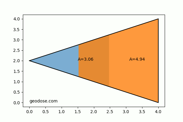 |
| Figure 5. Golden Section Search application. Splitting polygon into two parts with equal area |
That's all this post about Golden Section Search. We had discussed how the Golden Section Search works, implemented the method in Python to find an extremum value and discussed two application examples of this method. I hope those two examples could give you an idea how to apply the Golden Section Search method to solve a problem. I'm sure there are many more. Thanks for reading!
