Dynamics and Causes of Sea Level Rise in the Coastal Region of Southwest Bangladesh at Global, Regional, and Local Levels

Abstract

Global greenhouse gas emissions have caused sea level rise (SLR) at a global and local level since the industrial revolution, mainly through thermal expansion and ice melting. Projections indicate that the acceleration of SLR will increase in the near future. This will affect coastal and deltaic populations worldwide, such as in Bangladesh, where almost half of the population resides in regions lower than 5 m above sea level. This study found three coastal tidal gauges and five deltaic gauge stations, which showed increases in SLR at greater rates than the regional and global averages. This research also used satellite altimetry data to analyze regional and global SLR averages in the recent past and the 21st century. There is a trend towards increasing sea level based on results from three tide gauge stations: Char Changa with 7.6 mm/yr, Hiron Point at 3.1 mm/yr from 1993 to 2019, and 14.5 mm/yr at Cox’s Bazar from 1993 to 2011. Based on the linear trend from these time frames, it is projected that SLR in Char Changa will increase by 228 mm from 2020 to 2050, and by 608 mm by 2100, at Hiron Point by 93 mm in 2050 and 248 mm by 2100, and at Cox’s Bazar by almost 435.7 mm by 2050, and more than 1162 mm by 2100. Based on an average from satellite altimeters, assuming a linear increase in SLR, the Bay of Bengal shows an increase of 0.4 mm compared to the global trend. Other river delta stations in the study area also show increasing SLR, specifically, at Kalaroa, Benarpota, Kaikhali, Tala Magura, and Elarchari. Kalaroa and Benarpota show the highest, with SLR of >40 mm/yr. It is also observed that increasing SLR trends are far higher than coastal tide gauges, indicating that physical processes in the delta region are affecting SLR, further contributing to either an increase in water volume/SLR or activating land subsidence. This is partly due to the subsidence of the delta as a result of natural and anthropomorphic effects, as well as an increase in Himalayan glacier melting due to global warming. This indicates that Bangladesh coastal areas will soon experience a far greater SLR than the rest of the Bay of Bengal or other global coastal areas.

1. Introduction

The rise in average global surface temperature in the later part of the 21st century (2081–2100) is forecast to range between 1.5 °C and 2 °C, along with excessive rainfall occurrences, warming of the world’s oceans, and a sea level rise (SLR) of 8–16 mm/yr [1,2]. The continuous trend of greenhouse gas emissions (GHGs) will contribute to temperature rise, increasing the probability of unchangeable consequences for the environment, and exacerbating prevailing threats while creating new perils [1,2]. At the same time, the atmosphere is experiencing higher concentrations of carbon dioxide (CO₂), methane (CH₄), and nitrous oxide (N₂O) than in the last 800,000 years, and projections for sea level indicate a continuous increase even after GHG emissions decline [1,3]. During the 20th century, global SLR experienced an increase of approximately 2 mm/yr, which is comparatively greater than in the last 3000 years [1]. From 1901 to 2018, the worldwide average sea level rose by 0.20 (0.15 to 0.25) mm and the regular proportion of sea level rise was 1.3 (0.6 to 2.1) mm/yr from 1901 to 1971, swelling to 1.9 (0.8 to 2.9) mm/yr from1971 to 2006, and additional swelling to 3.7 (3.2 to 4.2) mm/yr from 2006 to 2018 [1,4,5]. However, the precise projection of future SLR needs continuous observation and modeling of the integrated ice–ocean–land–atmosphere–climate dynamics [6,7]. Thus, a strong initiative is needed to have reliable data tracking from satellite altimeters and independent ocean observation systems. Along with this, studies from various disciplinary initiatives are necessary to deal with serious issues which include improving the historical recording of SLR and ocean temperature increase, isolating geophysical processes from sea level increase signals, as well as the comprehensive perception of the interactive relationship between oceanic surface and ice sheets [6,7].

GIA (global isostatic adjustment) is a modeling procedure that is related to the adjustment of Earth’s lithosphere and viscous mantle material to past changes in ice loading since the last glaciation [8]. GIA can, thus, contribute to important meridional differences in mean sea level (MSL) change, as is seen in sea level projections for tide gauge locations in the UK [9,10] and Scandinavia [11]. The spatial patterns for GIA in the tropics feature more homogenic and much smaller contributions to local MSL change compared to high latitudes. The contributions from GIA in the South Asia Region to overall sea level rise are generally insignificant [12].

As a result of global warming, SLR is driven by two primary mechanisms. First, glaciers and ice sheets melting at faster rates contributes to the increase in large volumes of freshwater into the oceans. Secondly, the volume of water in the oceans is increasing due to the expansion of water from the rising temperature. A third minor mechanism is the net transfer of water from freshwater lakes and rivers to oceans [1,13].

However, the rate and magnitude of SLR will not be equally distributed among the world’s coastal regions. Coastal regions, for instance, experience subsidence due to sediment compression from construction loading, soil erosion, and extraction of groundwater, natural gas, and petroleum resources [14]. Adverse outcomes of SLR include increased flood risk, loss of coastal buffers to hurricanes and flooding, exposed coastal waters to waste stored on land, saltwater intrusion into freshwater aquifers, as well as economic losses [3,15,16,17]. Furthermore, several nations experiencing the highest repercussions of SLR are not the primary emitters of GHGs. Bangladesh is ranked 162nd of 199 nations by the World Bank with regards to CO₂ release, revealing exceptionally disproportionate consequences of climate change [18,19]. Moreover, resettlement efforts are severely hampered by the turbulent geopolitical atmosphere in South Asia, which will be exacerbated by climate change and SLR [20,21,22,23]. These circumstances underscore the urgent need to diagnose and understand the dynamics of sea level rise in Bangladesh.

Furthermore, one of the most significant casualties of climate change and SLR is reported in Bangladesh, as approximately half of its population resides 5 m below the sea level and is the world’s sixth top calamity-stricken nation [23,24,25,26,27]. Due to Cyclone Bhola in 1970, Cyclone Sidr in 2007, Cyclone Aila in 2009, Cyclone Amphan, in May 2020, and the great flood of 1998, millions of people in Bangladesh have been rendered homeless, with hundreds of thousands of casualties [28,29,30,31,32,33,34]. In the near future, SLR will lead to the disappearance of 17% of the territory of Bangladesh, create 20 million refugees, and 220,000 km² of land will be submerged following a projected SLR of 1500 mm to take place within 150 years (According to CGTN, new research assumes that SLR will create 37 million refugees in Bangladesh) [33,34].

The impact of sea level rise in the southwest coastal region of Bangladesh (SWCRB) is exacerbated by phenomena such as floods, eroding coastlines, increased storm frequency and intensity, rising water tables, saltwater intrusion into aquifers, and ecosystem changes [35]. Simultaneously, the SWCRB receives freshwater and sediments from northern glaciers in the Himalayas that flow into the Ganges. Based on global warming predictions, Bangladesh will experience a dwindling glacial landscape outside the global level that would cause an SLR in the Bay of Bengal and its river delta [35,36].

It is also essential to observe the sea level and its fluctuations, especially along coastal areas due to the number of inhabitants occupying these areas. To do this, self-recording tide gauges (TGs) were used to gather the first historical sea records in the mid-18th century. In this study, to assess coastal SLR changes, tide gauge (TG) records serve as the main source of available information, as they were designed to measure Regional Sea Level (RSL) at their locations [37]. Thus, TG measurements also record Absolute Sea Level (ASL) changes that reflect local vertical land movements in geoid changes. In our analyses, annual averages of TG data were used to identify SLR in the Bay of Bengal. The tide gauge data for all station on the Bangladesh coast are limited by short recording periods, missing data (from certain years), and station instabilities. The three stations that provide data for about two decades without major interruptions are: (a) Hiron Point in the Sundarbans mangrove forest area (southwestern Bangladesh), (b) Char Changa in the Meghna estuary (central Bangladesh), and (c) Cox’s Bazar on the southeast coast. The original tide gauge data are monitored and collected by the Government of Bangladesh Inland Waterways and Transportation Authority (BIWTA), while the tide gauge data for the Ganges Delta were obtained from the Bangladesh Water Development Board (BWDB) [38,39].

Tide gauges have been the standard method to measure coastal sea level changes. The last few decades, however, have seen advancements in space-borne radar altimetry that provides new outlooks on global sea level changes. The use of satellite altimetry to monitor sea level was revolutionized when the US/French mission TOPEX/Poseidon (CNES/NASA) was launched in August 1992 [40]. Using a geocentric terrestrial reference frame to measure the sea surface height and estimate sea level temporal variation is a main advantage resulting from the satellite radar altimetry mission [41,42]. However, the in-situ sea level temporal variation is measured from TG references to a particular ground station [43]. The readings provided by the satellite altimetry provide more precise measurements in a low temporal sampling rate, and wide resolution, with a well-defined geocentric reference frame, compared to the low spatial and high temporal resolutions of tide gauges. Due to the satellites taking periodic measurement, usually 10–35 days, the altimeter measurements can determine global mean sea level change superiorly to tide gauges. This is because tide gauges describe high-frequency variations, such as tsunamis or any extreme sea level event that has long-period processes. Spatial and temporal coverage have been provided by satellite altimetry for almost a decade, providing important information on a one-month to several-years’ time scale on mean sea level changes [39]. As such, it is essential to study the long-term changes in sea level on the coastal zone, as much of the world’s population resides in these areas, as well as for other environmental and socio-economic reasons [44,45].

Our study showed variations in sea level and trends in the Bay of Bengal and globally, using multi-mission satellite altimeters. This research aims to determine the future sea level rise in Bangladesh and its coastal river deltas, which will be compared to global sea level rise and sea level rise in the Bay of Bengal, its river deltas, and its impact on local, regional, and global levels.

Relative Sea Level Rise

Relative sea level rise (RSLR) is a reaction to climatic as well as non-climatic contributors and differs with situations [46,47]. RSLR depends on local shifts in water flow, air flow, saline concentration, and water temperature [48]. The relative sea level is defined by the limit of the subsiding delta plain (considering that the delta is close to or at the base level), and the seaward gradient of accommodation. The pattern of subsidence is found for the Ganges–Brahmaputra–Meghna Delta (GBMD) using its Holocene relative sea level history. The results show that there is Holocene subsidence over the delta, and that it increases from the Hinge Zone (landward) to seaward from <0.2 mm/yr to 2 ± 0.7 mm/yr in the middle fluvial delta and, in the lower tidal delta, to 4 ± 1.4 mm/yr. This provides us the opportunity to create a first millennial-scale map of the GBMD on its subsidence pattern [49,50]. RSLR is more rapid than typical global patterns in collapsing coastlines, inclusive of deltaic regions such as the Mississippi, the Nile, and the great deltas of South and East Asia (e.g., the Ganges deltaic region in Bangladesh) [48]. Nevertheless, RSLR is attributable to a more neighboring or regional extent, such as crustal deformation, tectonic shifting, volcanic activity, ground subsidence from nature-induced reasons (e.g., sediment filling rivers and deltaic areas), or human actions (groundwater or oil/gas extraction). Some communities and nations may face faster or higher RSLR than the global average rate due to complicated interplay between geomorphological and ecological features of the coastal setting, as well as mitigating capacity [50,51]. Due to this, understanding the extent of RSLR in coastal environments is essential. For instance, the Bay of Bengal was created after the India–Asia collision, thickening of the Tibetan Plateau, and the uplift of the Himalayas. Furthermore, the Bengal Basin is divided into three geotectonic provinces: 1. The northwest consists of a stable shelf, and the west has a passive-to-extensional continental margin. 2. The center has a deep basin. 3. The east has a fold belt, namely, the Chittagong Tripura Fold Belt (CTFB) [52]. It is argued, however, that the northern Bay of Bengal is considered “thin continental” after it endured continental rifting and was exposed to volcanic activity from the Kerguelen hotspot [53]. When it comes to the deposition of sediment in the Bay of Bengal, it has been speculated that tectonic cycles or stages regarding the interaction and collisions of major plates plays a role. There have been five phases thus far: 1. Syn-rift stage 2. Drifting stage 3. Early collision stage 4. Late collision stage 5. Latest collision stage. Furthermore, sediments originating from Himalayas and the Indian Peninsula that are transported by the Ganges and Brahmaputra Rivers are considered to be mostly detrital than biogenic [52]. As the Bengal Basin accumulates a large amount of sediment through faulting, folding, and compaction, the Bengal Basin margin shows a prograde of more than 300 km in the last 35 million years. When it comes to human interactions, the geological exploration in the Chittagong Tripura Fold Belt (CTFB), for instance, has increased due to more earthquakes and structural complexities (i.e., thrust faults and mud volcanoes) [54]. Furthermore, national and international oil and gas companies have conducted seismic surveys and drilling due to the presence of anticlinal folds and faults related to gas seepages [52].

One of the major instances of relative sea level changes is seen in the vicinity of the Bay of Bengal, depending moderately on changes in the measurements of the ocean where sea level increases at a risky rate in comparison to land [55,56,57]. South Talpatti Island, or Purbasha, was a coastal island in Shyamnagar Upazila of Satkhira district in Bangladesh. However, due to SLR in Bangladesh, South Talpatti was lost to the sea in the Bay of Bengal in the late nineties [58,59]. This indicates that the southern part of Bangladesh, especially Gabura and Padmapukur unions, will be submerged. Both of these unions were under water at the time of Cyclone Aila. Moreover, the inhabited island of Lohachara, located at the mouth of the Hooghly River in India, adjacent to the Ganges Delta, gradually sank in the 1980s [60,61,62]. During the previous 30 years, the relative sea level has increased quicker than the global mean sea level (GMSL) (high confidence) in the area near Asia. Within the timeframe 1984 to 2015, the entire region of the coastal neighborhood diminished and the coastline attenuated; however, some coastlines drifted towards the Russian Far East, East Asia, and Southeast Asia such as the Southern Coastal region in Bangladesh [48,55,63].

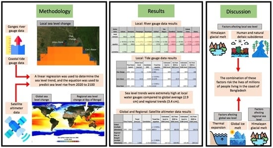
2. Study Area and Methodology

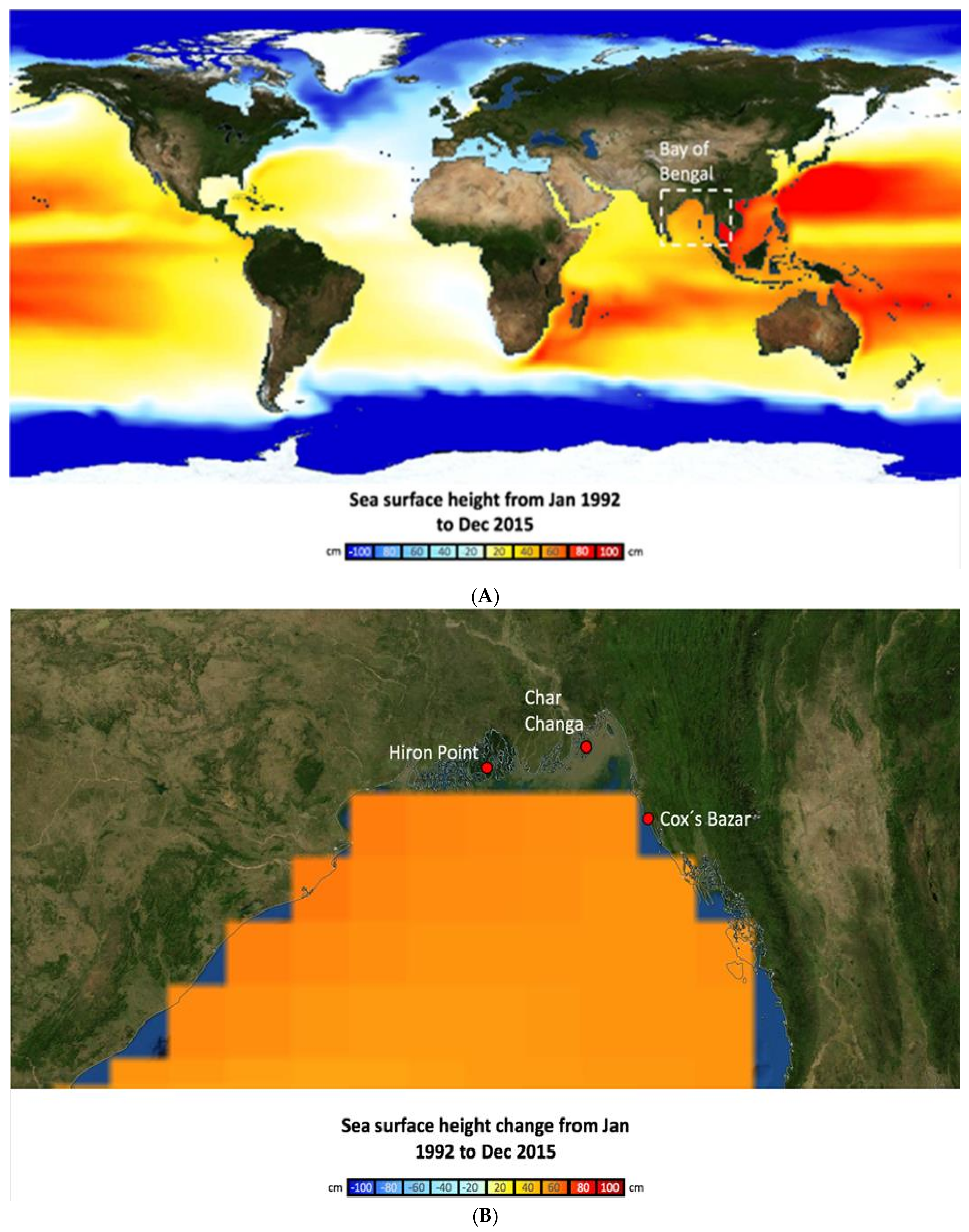
2.1. Study Area

The study area is within the southwestern part of Bangladesh between 22.3306′ N and 89.1028′ E, encompassing the entire Sundarbans (Figure 1A,B) [62,64].

Delta sediments form a shallow area that extends about 200 km south from the coastline. In the western part of the Indian Ocean, beyond the narrow coastal zone, the seabed quickly drains to a depth of 2000 m or more. In the east, the Andaman Sea forms a shallow water area [65,66]. The largest fluvio-deltaic-to-shallow marine sedimentary basin of the world is the Ganges–Brahmaputra–Meghna (GBM) Delta. This basin receives inflow from the Ganges in the northwest, and the Brahmaputra from the northeast, while the Meghna provides input from flowing into the Brahmaputra (after entering the Sylhet Trough and part of the Tripura Hills), and finally, into the Bay of Bengal. From the Bengal Basin, it is estimated that about 1.1 gigatons (GT) of cumulative sediments are dispersed into the Bay of Bengal, resulting from the largest submarine fan in the world, the Bengal Fan [67,68]. The Himalayas shed sediments into the GBM Delta, the source of most of the sediments, while the Himalayan front, Shillong Plateau uplift in the north, and the accretionary fold belt in the east can create tectonic influences on the GBM Delta [67]. Flexural subsidence, faulting, folding, and localized compaction are sources for less than half of the total sediment trapped in the Bengal Basin [68]. This accumulated sediment has resulted in a prograde of more than 300 km since the Eocene (35 Ma) in the entire Bengal Basin [67,68].

2.2. Methodology

Sea level is measured using two main approaches: tide gauges and satellite altimeters. Tide gauges measure low and high tides by utilizing manual and automatic sensors. Satellite altimeter radar measurements are performed using precision-based spacecraft orbits to determine the surface altitude with exceptional accuracy [69,70]. The mean tide level at any location is the average of all high and low water levels at that location over a long period of time. In sea level analyses, there are some advantages to using mean tide level as a locus level instead of mean sea level (MSL) [71].

The daily high SLR/water level and daily low SLR/water level (in meters (m)) were obtained from the Government of Bangladesh Inland Waterways and Transportation Authority (BIWTA) tide gauge data. Mean SLR was calculated by averaging the daily high and low SLR in m, which was further converted to mm scale (

Table 1. Data from three tide gauge stations from the Bay of Bengal at Hiron Point, Char Changa, and Cox’s Bazar (primary data were collected from Government of Bangladesh Inland Waterways and Transportation Authority (BIWTA)).

Year (Char Changa)	Latitude	Longitude	Lowest	Highest	Average	Year (Hiron Point)	Latitude	Longitude	Lowest	Highest	Average	Year (Cox’s Bazar)	Latitude	Longitude	Highest
1993	21.78	89.47	0.58	3.82	2.20	1993	22.23	91.05	0.28	3.20	1.74	1993	21.45	91.83	3.85
1994	21.78	89.47	0.52	3.98	2.25	1994	22.23	91.05	0.26	3.25	1.75	1994	21.45	91.83	3.75
1995	21.78	89.47	0.67	4.12	2.39	1995	22.23	91.05	0.37	3.30	1.84	1995	21.45	91.83	3.99
1996	21.78	89.47	0.66	3.90	2.28	1996	22.23	91.05	0.38	3.29	1.84	1996	21.45	91.83	3.91
1997	21.78	89.47	0.58	4.03	2.30	1997	22.23	91.05	0.21	3.22	1.72	1997	21.45	91.83	3.83
1998	21.78	89.47	0.64	4.18	2.41	1998	22.23	91.05	0.41	3.33	1.87	1998	21.45	91.83	3.91
1999	21.78	89.47	0.70	4.08	2.39	1999	22.23	91.05	0.29	3.27	1.78	1999	21.45	91.83	3.96
2000	21.78	89.47	0.61	4.07	2.34	2000	22.23	91.05	0.43	3.44	1.93	2000	21.45	91.83	4.00
2001	21.78	89.47	0.67	3.96	2.32	2001	22.23	91.05	0.48	3.44	1.96	2001	21.45	91.83	3.95
2002	21.78	89.47	0.66	4.07	2.36	2002	22.23	91.05	0.33	3.28	1.80	2002	21.45	91.83	4.01
2003	21.78	89.47	0.55	3.72	2.14	2003	22.23	91.05	0.41	3.38	1.89	2003	21.45	91.83	3.92
2004	21.78	89.47	0.52	3.79	2.16	2004	22.23	91.05	0.34	3.41	1.87	2004	21.45	91.83	3.85
2005	21.78	89.47	0.53	3.78	2.15	2005	22.23	91.05	0.37	3.37	1.87	2005	21.45	91.83	4.02
2006	21.78	89.47	0.56	3.86	2.21	2006	22.23	91.05	0.26	3.27	1.77	2006	21.45	91.83	3.97
2007	21.78	89.47	0.68	4.02	2.35	2007	22.23	91.05	0.29	3.39	1.84	2007	21.45	91.83	4.07
2008	21.78	89.47	0.70	4.02	2.36	2008	22.23	91.05	0.41	3.48	1.95	2008	21.45	91.83	4.07
2009	21.78	89.47	0.74	4.00	2.37	2009	22.23	91.05	0.43	3.52	1.97	2009	21.45	91.83	4.11
2010	21.78	89.47	0.70	4.05	2.38	2010	22.23	91.05	0.41	3.34	1.88	2010	21.45	91.83	4.15
2011	21.78	89.47	0.68	4.04	2.36	2011	22.23	91.05	0.37	3.29	1.83	2011	21.45	91.83	4.07
2012	21.78	89.47	0.73	4.07	2.40	2012	22.23	91.05	0.36	3.33	1.84	-			-
2013	21.78	89.47	0.60	3.97	2.29	2013	22.23	91.05	0.40	3.32	1.86	-			-
2014	21.78	89.47	0.84	4.15	2.50	2014	22.23	91.05	0.37	3.40	1.88	-			-
2015	21.78	89.47	0.78	4.13	2.45	2015	22.23	91.05	0.35	3.33	1.84	-			-
2016	21.78	89.47	0.75	4.15	2.45	2016	22.23	91.05	0.38	3.47	1.93	-			-
2017	21.78	89.47	0.79	4.33	2.56	2017	22.23	91.05	0.34	3.41	1.87	-			-
2018	21.78	89.47	0.76	4.24	2.50	2018	22.23	91.05	0.30	3.36	1.83	-			-
2019	21.78	89.47	0.64	4.17	2.40	2019	22.23	91.05	0.28	3.47	1.87	-			-

). Yearly mean SLR was calculated from these data and plotted in Excel. Finally, trends of MSL were calculated by linear regression with the regression coefficient sea level information at Sundarbans/Hiron Point and Char Changa from 1993 to 2019 and at Cox’s Bazar from 1993 to 2011 obtained, and both the lowest and highest tide records were retrieved (Figure 2A–C).

For Hiron Point, the highest tide value was considered from March and the lowest from August. The lowest and highest tide values were considered for February and August for both Char Changa and Cox’s Bazar. Then, for Hiron Point and Char Changa, the average between the lowest and the highest point was considered as the average annual SLR value, and only the highest tide record was used as the annual value for Cox’s Bazar, due to unreliable low tide records.

Tide gauge data for the Ganges Delta were obtained from the Bangladesh Water Development Board (BWDB). Metric data from the BWDB were available for 10 stations, with a data series from 1968 to 2019 (

Table 2. Data from 10 tide gauge 10 stations from the Ganges Delta (primary data were collected from the Bangladesh Water Development Board (BWDB)).

Data BWDB	Kalaroa	Benarpota	Protapnagar	Basantapur	Kaikhali	Tala Magura	Chandkhali	Elarchari	Kobadak Forest	Shakra
Latitude	22.87		22.39	22.46	22.19	22.73	22.52	22.66	22.22	22.63
Longitude	89.05		89.19	89.03	89.08	89.27	89.25	89.05	89.31	88.95
Year	Average	Average	Average	Average	Average	Average	Average	Average	Average	Average
1968	1527.89	913.85	567.36	838.18	563.74	619.38	657.13	1529.89	343.53	1030.49
1969	1279.15	806.88	579.05	752.12	514.53	607.27	577.26	1659.47	255.51	1088.18
1970	1566.59	1000.82	628.79	802.01	588.03	523.10	532.79	1087.67	305.44	1148.69
1971	1705.26	969.78	388.94	785.92	540.31	572.65	548.63	1402.27	334.85	1233.60
1972	1045.22	682.91	560.60	705.82	533.71	493.55	543.09	1286.23	266.49	996.73
1973	1293.06	765.27	656.79	824.48	532.23	569.12	572.29	1554.44	302.78	980.34
1974	1357.07	808.53	591.01	686.57	668.48	754.71	697.34	1335.00	383.81	927.81
1975	1275.89	780.21	572.85	908.60	609.77	550.44	624.35	1704.02	353.40	822.71
1976	1241.86	642.79	524.21	1167.65	1419.70	310.33	624.86	1683.58	302.16	1021.16
1977	1331.37	789.60	588.42	1193.64	1668.00	575.45	652.51	1564.43	142.79	1059.70
1978	649.44	636.54	415.36	838.89	451.11	597.28	403.45	1600.52	298.63	1527.30
1979	1712.67	874.36	467.49	1160.55	392.36	1144.42	805.58	1567.53	349.36	1759.69
1980	1518.58	760.46	419.02	1080.30	496.20	994.74	711.84	1579.56	339.43	1855.33
1981	1816.70	852.62	748.79	1124.03	549.62	899.73	702.41	1519.89	416.33	1718.40
1982	1133.10	691.83	350.49	961.55	464.73	141.50	581.69	1586.99	331.20	455.56
1983	1290.90	879.98	−81.25	799.07	397.38	653.56	675.29	1641.07	413.97	956.51
1984	1700.44	935.71	−88.52	855.89	808.55	672.87	666.21	1515.33	456.37	930.81
1985	1372.66	754.90	64.26	803.49	793.44	564.23	598.04	2056.00	372.63	924.70
1986	1834.37	983.37	−12.67	747.22	742.59	631.41	566.47	1969.01	394.21	901.99
1987	1734.32	905.40	151.18	784.32	643.14	581.30	730.29	2040.64	496.15	858.79
1988	1732.86	994.78	335.31	900.05	522.14	805.77	667.55	2010.27	399.32	1159.39
1989	1589.96	949.67	498.32	866.04	820.92	876.33	438.74	1883.10	522.07	848.96
1990	1828.48	997.44	270.38	886.25	821.85	937.61	625.59	1865.23	600.70	880.15
1991	1735.01	981.60	329.25	784.78	785.64	1274.89	567.86	1752.11	442.23	865.22
1992	2479.36	1072.17	568.41	788.73	784.55	183.35	585.08	1638.68	281.69	541.32
1993	2176.78	1337.95	342.66	804.12	805.32	827.93	446.59	1272.42	325.71	834.87
1994	1889.36	1328.38	277.89	777.01	557.97	671.29	540.40	1793.14	232.47	747.05
1995	2304.25	1477.07	198.75	842.45	742.64	658.44	196.01	1825.93	138.27	781.49
1996	2647.88	1454.39	48.20	778.14	927.32	674.11	309.08	2144.30	182.24	899.85
1997	2530.64	1481.29	66.89	691.71	726.33	670.75	572.11	2148.46	16.01	748.45
1998	2509.67	1266.26	−172.55	794.10	814.99	784.44	578.29	2419.32	−130.89	880.55
1999	2597.43	1537.21	−299.93	905.36	849.25	752.15	579.08	2552.59	−42.00	898.19
2000	1935.81	1795.58	29.60	968.90	844.21	767.82	611.81	2685.87	−67.77	1055.65
2001	2823.40	1559.10	97.34	855.89	825.78	643.26	676.10	2455.96	−337.12	917.13
2002	2380.10	1519.29	370.98	862.07	813.40	544.03		2342.51	308.86	890.71
2003	2629.24	1080.77	202.69	933.16	787.06	444.80		1744.33	180.93	867.64
2004	2880.26	1233.98	363.43	821.58	777.26	846.49		1992.79	−311.65	949.47
2005	3391.31	1382.43	118.53	714.00	851.40	996.15		2161.86	−175.15	1203.61
2006	2799.31	1424.37	761.31	717.53	806.12	750.72		2032.76	−279.02	1177.83
2007	2879.91	1166.62	1124.29	876.79	711.85	−31.98		2740.13	−82.51	743.25
2008	3193.69	1647.87	759.71	869.00	870.13	224.62		3447.50	−289.85	761.57
2009	2304.01	1560.83	575.12	795.97	897.74	642.56			−306.34	846.13
2010	1870.99	1789.15	395.86	945.67	981.10	454.66			−377.69	930.70
2011	2273.29	2421.52	416.34	1104.51	1007.99	829.60				924.81
2012	2274.03	2761.69	309.34	1155.52	1027.43	511.34				1105.99
2013	2983.97	3237.05	291.93	1270.08	1034.08	1621.39				1069.86
2014	3406.19	2857.87	439.44	1114.84	986.51	2824.77				983.64
2015	3438.19	2751.72	765.30	896.21	1031.63	1833.07				971.21
2016	3470.18	3232.11	868.99	888.36	1015.98	1478.88				1101.93
2017	3169.51	3712.50		772.99	996.15	1298.65				943.99
2018	2946.99			700.60	954.79					893.25
2019	2446.49			559.94	792.66					650.80

). The list of stations includes Kalaroa, Benarpota, Protapnagar, Basantapur, Kaikhali, Tala Magura, Chandkhali, Elarchari, Kobadak Forest Office, and Shakra, which include timeframes of 52, 50, 49, 51, 52, 51, 49, 34, 43, and 39 years, respectively. The monthly data were taken into consideration for tidal documentation if a minimum of 15 days of data were obtained, and yearly data were considered if a minimum of 11 months of data were obtained. Time extent of these statistics is significantly of high quality. Usually, data from the past 20 years were examined for SLR tendency assessment and the data quality verified before scrutiny [51]. The inaccuracy in tidal statistics was rectified manually. In case of an over-inference of tidal rank, flawed data were removed from the dataset. Some impractical values, such as the same value for high and low tides, were removed from the dataset before obtaining a sea level rise trend (Table 2). Some data points were identified as erroneous and removed manually.

In this study, we showed how Global Navigation Satellite System (GNSS)-derived vertical velocities contribute to the correction of tide gauge (TG) measurements used for sea level rise estimation in the Ganges–Brahmaputra–Meghna Delta (GBMD) [72,73,74]. At the Ganges–Brahmaputra–Meghna Delta (GBMD), vertical land motion (VLM) and GNSS (co-located) are used when estimating the geocentric sea level rise. TGs use a land-based monitored geodetic benchmark to measure the height of water. Thus, VLM can be determined using GNSS-based methods. The absolute geocentric sea level trend is the conversion of the TG correction of relative sea level heights and GNSS vertical velocities from the same location [72,73,74].

2.3. Satellite Imagery Retrieval

Satellite data were retrieved from the Laboratory for Satellite Altimetry [75,76,77], including data from TOPEX, Jason -1, -2, -3, and multiple altimeters, which were averaged to create a 1992 to 2020 table [5,76,77,78,79,80,81,82,83,84,85]. Global and local level changes provide a method for evaluating the performance of climate models This was used to measure global average and regional SLR; the regional data were obtained from the average altimetry values of the Bay of Bengal. To visually analyze global and regional SLR, screenshots were obtained from the JPL ECCO server (2020) [5,78,79,80,81] which show the change in sea surface topography from 1992 to 2015 [79,80,81,82,83].

2.4. SLR Change Verification and Land Subsidence Projection Using CMIP5 Model

The Norwegian Earth System Model (NorESM1-EM) from CMIP5 (Coupled Model Intercomparison Project Phase 5) was used to compare the mean SLR of regional and global areas. For the mean regional SLR, the mean SLR for the Bay of Bengal was used, and projections of land subsidence were analyzed to determine their relationship. SLR projections (the representative concentration pathways (RCPs) data were downloaded from cds.climate.copernicus.eu (accessed on: 22 December 2021) [82,83,84] and the mean SLR for the Bay of Bengal was simulated using the Global Climate Model (GCM) NorESM1-ME from 2006 to 2100. The estimates were taken from the figures from 1980 to 2005. The GCM model figures were in the Network Common Data Form version 4 (NetCDF4) pattern. The data utilizing the Climate Data Operator means were separated and the Python language was employed to plot the RCP estimates [82].

3. Results

The results from the three tide gauge stations indicate a trend towards increasing sea level, with Changa at 7.6 mm/yr and Hiron Point at 3.1 mm/yr from 1993 to 2019, and a staggering Cox’s Bazar at 14.5 mm/yr of SLR from 1993 to 2011 (Figure 2,

Table 3. Timeframe, sea level rise trend, correlation, trend line equation, and estimated level in 2050 and 2100, and sea level rise from 2020 to 2050 and 2100 for tide gauges at Char Changa, Cox’s Bazar, and Hiron Point. Cox’s Bazar shows a significantly higher rate of SLR through the 21st century, with >1 m of rise during a period of 80 years (Data Source: BIWTA, 2020).

Time Frame (Years)	Water Level Trend (mm/yr)	Correlation (R2)	Trend Line Equation	Estimated Level in 2050 (mm)	SLC from 2020 to 2050 (mm)	Estimated Level in 2100 (mm)	SLC from 2020 to 2100 (mm)
Char Changa 1993–2019	7.6	0.3066	y = 0.0076x − 12.881	2699	228	3079	608
Cox’s Bazar 1993–2011	14.52	0.6097	y = 0.0145x − 25.1079	4665	435.7	5391	1162
Hiron Point 1993–2019	31	0.1466	y = 0.0031x − 4.4224	1932.6	93	2087.6	248

). A significant correlation exists for Car Changa, with an R² value of 0.307, and an extremely significant correlation exists for Cox’s Bazar, with an R² of 0.610. Based on the linear trend line from these time frames, it is projected that SLR in Char Changa will increase by 228 mm from 2020 to 2050, and 608 mm in 2100, Hiron Point by 93 mm in 2050 and 248 mm by 2100, and Cox’s Bazar almost 435.7 mm by 2050, and more than 1162 mm by 2100, assuming a linear increase in SLR. Cox’s Bazar has an SLR projection similar to those in the intermediate–high region. The detailed statistical analysis are in Supplementary Materials.

According to the monthly average sea level data from 1993 to 2011, the MSL trend of Cox’s Bazar was +14.5 mm/yr. (R² = 0.6097). The increase in sea level from 1993 to 2011 was 206 mm. Using regression analysis, the trend of sea level rise was predicted (Figure 2, Table 3). As per the predictions, after 100 years, the sea level may rise by 1450 mm from the existing sea level.

Tidal statistics at the three-gauge locations on the coast of Bangladesh have shown an SLR of 4.0–7.8 mm/yr for 1977–1998 [61,86,87]. This is significantly greater than the pace of global SLR during the 19th century, i.e., 1.7 ± 0.3 mm/yr [1,3]. SLR statistics retrieved from the three tidal checkpoints in the SWCRB reveal that Hiron Point has an increasing SLR of 3.1 mm/yr, Char Changa of 7.6 mm/yr, and Cox’s Bazar of 14.52 mm/yr, showing a significant increase from 5.5 and 7.5 mm for the same regions from 1970 to 2005 [86,87]. Verification of SLR statistics from 10 tide gauge watch points within the coast of Bangladesh for intermittent time points (14–44 years) details a mean SLR of up to 38.8 mm/yr, near the central coastal belt. These trends can be derived from a number of factors, as shown in Table 3 and Table 4.

Several of the stations show increasing SLR, specifically, Kalaroa, Benarpota, Kaikhali, Tala Magura, and Elarchari, (Figure 3 and Table 4). Most of them have very high rates of SLR, especially the first two, which show a rise in SLR of >40 mm/yr. At the same time, the river gauges show significant correlations of SLR data among the given stations, in particular for Kalaroa and Benarpota, of >R² = 0.6 (Table 4). Two stations, Protapnagar and Basantapur, showed no significant SLR change or correlation, with a trend of <0.5 mm/yr. Chandkhali, Kobadak Forest, and Shakra showed a decrease, with −3.03 mm/yr, −13.59 mm/yr, and −4.92 mm/yr, respectively. Overall, this indicates that half of the stations’ SLR are increasing at rates between 7.27 mm/yr and 41.75 mm/yr, rates much higher than the three stations with their corresponding decreasing rates, suggesting general RSLR within the Delta. At the same time, increasing SLR trends are far higher than the coastal tide gauges, indicating that other physical processes within the delta region are affecting SLR, which could contribute to either an increase in water volume/SLR or active land subsidence.

Table 4. Trend in sea level rise, equation of the trend line, and correlation of 10 stations measuring sea level rise (SLR) at the Ganges Delta. The green color indicates positive SLR, red indicates negative SLR, and yellow indicates no significant trend. Four of the five positive SLR trend stations show a significant correlation with their timeframe, indicating more reliable predictions than those with little or no correlation. Data retrieved from BWDB.

Station Name	Kalaroa	Benarpota	Protapnagar	Basantapur	Kaikhali	Tala Magura	Chandkhali	Elarchari	Kobadak Forest	Shakra	Legend
Trend (mm/yr)	40.41	41.749	0.127	0.0898	7.2704	11.528	−3.0327	29.343	−13.59	−4.9207	Positive sea level change
Correlation	0.7241	0.665	0	0	0.2149	0.148	0.0644	0.578	0.533	0.081	No significant sea level change (<1 mm/yr)

Table 4. Trend in sea level rise, equation of the trend line, and correlation of 10 stations measuring sea level rise (SLR) at the Ganges Delta. The green color indicates positive SLR, red indicates negative SLR, and yellow indicates no significant trend. Four of the five positive SLR trend stations show a significant correlation with their timeframe, indicating more reliable predictions than those with little or no correlation. Data retrieved from BWDB.

Station Name	Kalaroa	Benarpota	Protapnagar	Basantapur	Kaikhali	Tala Magura	Chandkhali	Elarchari	Kobadak Forest	Shakra	Legend
Trend (mm/yr)	40.41	41.749	0.127	0.0898	7.2704	11.528	−3.0327	29.343	−13.59	−4.9207	Positive sea level change
Correlation	0.7241	0.665	0	0	0.2149	0.148	0.0644	0.578	0.533	0.081	No significant sea level change (<1 mm/yr)

The global data showed an increase of 2.94 mm/yr based on an average from satellite altimeters, with an extremely high correlation of 0.919 from 1992 to 2020, as seen in

Table 5. The timeframe, sea level rise (SLR) trend, correlation, trend line equation, estimated level in 2050 and 2010, and SLR from 2020 to 2050 and 2100 for global and regional sea surface topography from 1992 to 2020. The regional data are based on the Bay of Bengal region. Data from altimeters from TOPEX/Poseidon and Jason-1, -2, -3 were averaged to create the historical record. Data obtained from the Laboratory for Satellite Altimetry (2020a and 2020b) [76,77,78,80].

	Time Frame	Trend (mm/yr)	Correlation	Tread Line Equation	Estimated Level in 2050 (mm)	SLC from 2020 to 2050 (mm)	Estimated Level in 2100 (mm)	SLC from 2020 to 2100 (mm)
Global	1992–2020	2.935	0.9192	y = 2.9345x − 5869.4	146.325	88.035	293.05	234.76
Regional (Bay of Bengal)	1992–2020	3.366	0.3516	y = 3.3664x − 6733.6	167.25	100.992	335.84	269.312

. The trend is not constant across the globe, with polar regions showing decreasing SLR rates and places near the equatorial Pacific having the highest increasing rates, approaching up to 1000 mm in certain regions (Figure 4). The linear projection of global sea level change in 2050 indicates an SLR of 88.04 mm compared to 2020 and 234.76 mm by 2100 (Table 5).

The regional data show an increasing trend of 3.37 mm/yr, with a correlation of 0.352 (Table 5). The regional trend is higher by 0.4 mm than the global trend. Based on the map and graph (Figure 4 and Figure 5), higher regional levels exist along the coastal region of the Ganges Delta. The future trend for the region of the Bay of Bengal indicates a 100.99 mm rise from 2020 to 2050, and a rise of 269.31 mm from 2020 to 2100, which is higher than those of global values. However, both predictions have SLR trends where the regional trend is slightly higher than the global average and relatively mild compared to both the river and coastal tide gauges. Average river gauge trends are higher than global and regional trends, with two coastal gauges projecting a change of more than 1000 mm from 2020 to 2100. Only Hiron Point presented trends and future projections similar to those of regional and global ones.

The Bay of Bengal (regional data) and global data have a strong correlation of R² = 0.70 (

Table 6. Correlation of annual SLR data from global data, Bay of Bengal, Char Changa, Hiron Point, and Cox’s Bazar. The green color indicates correlations above R² = 0.2, yellow for R² = 0.1 and 0.2, and red for correlations less than R² = 0.1. Data retrieved from the Laboratory for Satellite Altimetry [76,77,78,88,89] and BIWTA.

	Global SLR	Bengal Bay SLR	Char Changa	Hiron Point	Cox’s Bazar	Legend
Global SLR	1	0.70	0.32	0.12	0.58	>0.2
Bengal Bay SLR	0.70	1	0.30	0.19	0.56
						0.1–0.2
Char Changa	0.32	0.30	1	0.04	0.23
Hiron Point	0.12	0.19	0.04	1	0.39	<0.1
Cox’s Bazar	0.58	0.56	0.23	0.39	1

); based on this timeframe, the lineal trend is similar for both regional and global data, but the trend for Bay of Bengal SLR is higher than that for the global average. Both the global and Bay of Bengal SLR have a correlation of R² = 0.32 and 0.30 with Char Changa, and 0.58 and 0.56 with Cox’s Bazar, respectively. Hiron Point only had a significant correlation, of 0.39, with Cox’s Bazar. This indicates that although the rates for local regions have higher SLR trends, the local changes in SLR are statistically consistent with the regional (Bay of Bengal) and global SLR patterns, except for Hiron Point.

3.1. Comparison with the CMIP5 Model

Under RCP 2.6, RCP 4.6, RCP 6, and RCP 8.5, the global MSL shows 0.30, 0.35, 0.37, and 0.48 m, respectively, in 2100. Furthermore, in the Bay of Bengal, the MSL is indicated to be higher than the global mean SLR. Under RCP 2.6, RCP 4.6, RCP 6, and RCP 8.5, the MSL shows 0.6, 0.7, 0.83, and 1.0 m, respectively, in 2011, in the Bay of Bengal (Figure 6)

3.2. Comparison with tide Gauge, Satellite Altimetry, and RCP, CIMP5

The results from the three tide gauge stations indicate a trend towards increasing sea level. It is projected that SLR in Char Changa will increase 228 mm from 2020 to 2050, and 608 mm in 2100. In Hiron Point, the increase is 93 mm in 2050 and 248 mm by 2100. In Cox’s Bazar, the increase will almost be 435.7 mm by 2050 and more than 1162 mm by 2100, assuming a linear increase in SLR. Global data also show increasing SLR, based on an average from satellite altimeters. The linear projection of global sea level change indicates an SLR of 88.04 mm in 2050 and 234.76 mm by 2100. The highest rate of increase is in the Equatorial Pacific, reaching almost 1000 mm in certain regions. For RCP, the values indicate that the MSL is higher regionally compared to globally. For instance, in the Bay of Bengal, RCP 2.6, RCP 4.6, RCP 6, and RCP 8.5, MSL shows 0.6, 0.7, 0.83, and 1.0 m, respectively, in 2100. Globally, RCP 2.6, RCP 4.6, RCP 6, and RCP 8.5 show 0.30, 0.35, 0.37, and 0.48 m, respectively, in 2100. Thus, it can be perceived that regional levels of SLR are almost higher than global levels.

4. Discussion

4.1. Sea Level Rise

This study compares historical and projected sea level change trends for the coast of Bangladesh, the Bay of Bengal, and globally. Averages were calculated using satellite altimeters, and tide and river gauges. The coast of Bangladesh presents the highest amount of sea level rise, which is a direct consequence of both natural and anthropogenetic events, related to subsidence in the deltaic environment, along with higher rates of glacial melt water from the Himalayas, resulting in sea level rise in the Ganges Delta. However, it is important to note that sea level rise will not be uniform, and the origins of glaciers may not experience sea level rise as extremely as other locations further from the melting source [88]. This is due to surface mass load self-gravitation where, near ice, water piles up due to the gravitational attraction, and flows away as the ice melts [88]. Thus, the melting of the Himalayan glaciers will, more than likely, contribute to more drastic increases in sea levels at locations further away from the Bay of Bengal. The Bay of Bengal region has rates higher than global averages due to the increase in Himalayan glacial meltwater, with a chance of reaching more than 200 mm by the end of the 21st century. However, due to the non-linear nature of sea level rise, projections can be expected to be much higher, threatening the lives of millions of people living in Bangladesh. The Bay of Bengal had a sea level trend of 3.4 mm and global averages of 2.9 mm per year. River delta sea level trends were of 3.1 to 41.7 mm per year, but many were above 7 mm per year. The sea level could rise by more than half a meter (500 mm) from 2020 to 2050, and from 2050 to 2150 by more than 1000 mm on the coast of Bangladesh, resulting in millions of Bangladeshi inhabitants possibly being submerged by 2100 (Table 3, Table 4, Table 5 and Table 6)

Sea level is eventually rising from west to east over the Bay of Bengal, and it progresses towards the North Bay of Bengal, causing subsidence over the coastal and adjacent regions. It has been projected that by 2040, the MSL over the Bay of Bengal will be 0.1 to 0.4 m under RCP 4.5. It will again increase by between 0.2 to 2 m during 2060. During 2080, the mean SLR range will be between 0.2 and 3.3 m. (Figure 6). Land subsidence over Bangladesh shows the highest magnitude over the southern and north-eastern parts as compared to the other parts. Barishal, Chattogram, and Khulna division will experience prominent SLR. Mainly, Khula, Satkhira, Pirojpur, Bhola, Patuakhali, Jalokathi, Barishal, Cox’s Bazar, Feni, Cumilla, Dhaka, Faridrur, Hobogonj, and Sylhet will face land subsidence during 2040 to 2080, according to the RCP 4.5 projection (Figure 7). Furthermore, the components and grain size of sediments play a role in subsidence [49]. In deltas, for instance, it was thought that plate-driven tectonic processes served as the main sources of subsidence [49]. However, compaction plays a more significant role on subsidence than before [89]. Thus, it is important to consider the compaction of strata (in deltas for instance), as this may also affect water levels [90]. As is evident from Figure 7, SLR determines the surface land area submergence, and land subsidence plays an important role, exacerbating the effect. It is also difficult to determine the true causes and patterns of subsidence due to the number of possible causes and patterns, including sediment loading, human activities, and decrease in soil from root decomposition [49,89].

As mentioned, sizes of locations, sediment composition, in-and-out fluxes of water and runoff, and grain sizes all play a role in how localities will be affected by a rise in sea levels. For example, subsidence factors in local areas occur faster than those over a greater area, and loose material in deltas easily compacts, resulting in slow sinking of the land and RSLR to rise 3.37 mm/yr (Table 5) [49,89]. The Ganges–Brahmaputra Delta, for instance, receives a lot of water and sediment input from the Himalayas, with an input of more than 1 billion tonnes/yr [49,90,91,92,93,94]. The subsidence levels for the lower delta showed 3 mm, the western ranged from 9 to 12.3 mm, and up 3.6 to 4 mm in the eastern, and it was also discovered that, within the first 10 years of the 21st century, immense flooding affected 85% of the largest deltas in the world, as shown in Figure 7 and Figure 8, [93,94,95,96,97]. Further, it is projected that the risk of flooding will increase by at least 50% by 2100 [49,93,94,95,96,97,98]. Thus, this delta is sinking so rapidly that the RSLR may reach 20 mm each year [96,97,98,99]. Subsidence rates for this delta range from 0 to >18 mm/yr [49,100,101].

Furthermore, the melting of glaciers may lead to a shortage of fresh water in the region, which will force humans to satisfy water needs from underground sources for both agricultural–industrial and domestic use. Excessive extraction of underground water will exacerbate land subsidence. Considering the impact of agriculture in water extraction, according to an article made in 2006 by the Ground Water Hydrology and the Bangladesh Water Development Board, 75% of the cultivated land is irrigated by groundwater; simultaneously, it also states that ~70 to 90% of abstracted groundwater is used for agricultural purposes [98,99,100]. A major cause of concern is that, since 2004, the groundwater in Bangladesh has not been recharging, as reported by the Bangladesh Agricultural Development Corporation in 2011. The rate of extraction was around 53 billion cubic meters per year, while the recharging rate was merely 50 billion cubic meters per year in 2011 [98,99]. The main occupation of the people in the Shyamnagar Upazila is agriculture and shrimp farming, resulting in an average land subsidence in Bangladesh of ~5 mm/yr [98,99,100].

Additionally, the areas submerged beneath the ocean will vary in different SLR situations. It has been confirmed that 0.5, 1, and 1.5 m of SLR will submerge ~4.3%, 8.4%, and 11.3% of the coastal regions of Bangladesh, and the number of impacted inhabitants will be 112 million [1,49,97,100,101,102,103]. The greatest risk of SLR is on the Sundarbans—the largest mangrove forest in the world—because it is not secured by coastal polders. It has been predicted that approximately 12%, 43%, and 60% of the Sundarbans will be submerged 0.5, 1, and 1.5 m, respectively (Figure 7 and Figure 8) [101,102,103]. Since the Sundarbans are significant from the biological, environmental, geological, and financi al perspectives for Bangladesh, its submergence with distinctive SLR circumstances will have devastating consequences.

Map shows the magnitude of land subsidence, with 3 mm for the lower delta, up to 9 mm of subsidence in the western delta, and up to 4 mm in the eastern delta. Additionally, subsidence values are 12.3 mm (in the western delta) and 3.6 mm (in the eastern delta). As is evident from Figure 8, SLR determines the surface land area submergence, and land subsidence plays an important role, exacerbating the effect.

Summary illustration of subsidence and compaction measurements for a section centered on the Brahmaputra incised valley is shown in Figure 9. Compacting sediments are in shades of brown to yellow, with brown indicating faster compaction. The methods applied to distinguish rates and their timescales and values are shown in green. The RSET and KHLC measure compaction from their base to the surface (upward arrows), while the other system measures subsidence below their base (downward arrows). At the bottom, values for long-term subsidence, shallow compaction, and short-term subsidence for the area around the polder, where we have all these systems, are given.

Though subsidence does play a role, it is important to consider the tide gauge and vertical land motion. For instance, tide gauges are affected by geocentric sea level and vertical land motion [102,103,104,105,106]. Thus, both are required to use satellite altimeters, as the observed sea level needs to be converted into a geocentric reference frame [93,104,105,106]. Local estimates of vertical land motion are also needed to derive an accurate estimate of ocean volume change, as mean vertical land motion at tide gauges is not the same as that of the basin [104].

4.2. Comparison between Global, Regional, and Local Sea Level Changes and Impacts

The coastal systems were considered to be affected mainly by higher sea levels. Sea levels will likely rise for many centuries at rates higher than that of the current century in the global and regional contexts [1]. It is also essential to compare regional sea level rise with the Bay of Bengal.

The satellite radar altimeter data in

Table 7. Regional sea level rise time series. Estimates for sea level rise were measured using satellite radar altimeter data retrieved from the Laboratory for Satellite Altimetry NOAA. Time series are available on TOPEX/Poseidon (T/P), Jason-1, Jason-2, and Jason-3 (launched in 1992), and altimeters launched in 1991 including T/P, Jason-1, Jason-2, Jason-3, ERS-2, GFO, and Envisat [76,77,78].

Region—TOPEX and Jason-1, -2, -3 Seasonal Signals Retained	MSL Trend mm/yr (1992–2022)
Pacific Ocean	2.8 ± 0.4
North Pacific Ocean	3.0 ± 0.4
Atlantic Ocean	3.1 ± 0.4
North Atlantic Ocean	2.7 ± 0.4
Indian Ocean	3.3 ± 0.4
Adriatic Sea	2.2 ± 0.4
Global Sea	3.0 ± 0.4
Baltic Sea	3.8 ± 0.4
Bay of Bengal	3.9 ± 0.4
Bering Sea	1.8 ± 0.4
Caribbean Sea	3.0 ± 0.4
Gulf of Mexico	3.9 ± 0.4
North Sea	2.8 ± 0.4
Mediterranean Sea	2.3 ± 0.4
Sea of Okhotsk	2.1 ± 0.4
Sea of Japan	3.0 ± 0.4
South China Sea	3.8 ± 0.4
Southern Ocean	3.2 ± 0.4
Yellow Sea	2.7 ± 0.4

show that sea level rise in the Bay of Bengal is higher than other regions. The statistical study of river gauges shows that five of the ten rivers measured are showing increased SLR at far higher rates than the global SLR averages (Figure 2, Figure 3, Figure 4, Figure 5 and Figure 6; Table 3, Table 4, Table 5, Table 6 and Table 7). Our data suggest considerably higher rates of SLR increase within the coast of Bangladesh as compared to that of either global rates or the rates for the Bay of Bengal. Both the tidal and the river gauges indicate far higher rates of SLR, with two having an order of magnitude with higher rates, looking at Figure 2, Figure 3, Figure 4, Figure 5 and Figure 6. RSLR can increase beyond the global mean sea level rise by an order of magnitude and is able to reach more than 100 mm/yr, and it is estimated that 50% of 33 deltaic regions have the potential to rise above global averages by 2100, according to the IPCC [1,2]. This explains the vast variation observed in our data, with rates considerably higher for sea level rise than the global average in the Bay of Bengal region.

The statistical study of river gauges shows that five of the ten rivers measured are showing increased SLR at far higher rates than the global SLR averages (Figure 2 and Figure 3; Table 4 and Table 5). The SLR in the river delta of the study area could be explained by the sinking and rising of the land, as the sinking of the land plays a role in the sea level rise in Bangladesh [1,49,94,100,101,102,103,104,105]. A probable 1.6 billion tones/yr of alluvial content streams towards Bangladesh through the Ganges and the Brahmaputra. Similarly, higher rates of ice melt in the Himalayan region would cause SLR in the Bay of Bengal and its river delta [103,104,105,106]. However, the subsidence of the deltaic landscape is considered to have been stabilized by the replenishment of dredges pushing towards a gross SLR and, in some regions, could rise due to an increase in river discharge by glacial meltwater. This could explain the three gauges with rising SLR trends and the two with no trends (Table 4). Our data suggest considerably higher rates of SLR increase within the coast of Bangladesh as compared to that of either global rates or the rates for the Bay of Bengal. Both the tidal and the river gauges indicate far higher rates of SLR, with two having an order of magnitude with higher rates Table 7 (Figure 2, Figure 3, Figure 4 and Figure 5). Strain from huge construction and engineering projects can equally give rise to compacted sedimentation and land sinking, such as in eastern Tokyo, Po Delta, Shanghai, and Bangkok [1,2,11]. It is also important to consider the size of the delta, as their size and composition rely on how much water is entering and leaving, with humans having an impact on this gradient [1,2]. RSLR can increase beyond the global mean sea level rise by an order of magnitude and is able to reach more than 10 cm/yr, and it is estimated that 50% of 33 deltaic regions have the potential to rise above global averages by 2100, according to the IPCC [1,2]. This explains the vast variation observed in our data, with rates considerably higher for SLR than the global average or the Bay of Bengal region.

In Figure 6, the RCPs indicate a global SLR projection in a non-linear fashion. Although the data are limited to local tide and river gauges, their trends will not be constant in the near future but are instead going to increase in a non-linear fashion, and are important to keep in mind, as flooding from tides can affect more areas.

As the global and the Bay of Bengal regional trends are correlated with local gauges in Bangladesh, it is safe to assume that the RCP non-linear trend will be reflected in the tide gauges, especially the coastal ones. Our global average linear projection falls below the lowest RCP on the lower standard deviation estimates of RCP 2.6 (Figure 6). This prediction is an underestimation of the other predictions, which would indicate that the regional Bay of Bengal and the coastal tide gauges are underestimating future trends. These are ultimately coupled, statistically, in our analysis based on Table 3, Table 5 and Table 6, where Cox’s Bazar and Char Changa have quite significant correlational values with respect to global averages and regional Bay of Bengal values.Furthermore, due to the exacerbation of many factors causing RSLR during the 21st century, the local SLR trends will have an even more pronounced exponential curve than their comparison with the RCP prediction in Figure 6. Therefore, both Char Changa and Cox’s Bazar, with estimates of more than half a meter for the former and over a meter for the latter in a linear trend based on the relatively little historical record, could expect a few meters (Figure 2 and Figure 3) of SLR for Cox’s Bazar and well over a meter for Char Changa. This situation is critical for Bangladesh, and the scarce local data from gauges have a relatively short temporal range, scarce locations of gauges, and a highly dynamic environment with multivariable sources of RSLR, which together reduce the possibility of a confident prediction of local SLR. The Table 8 provides a summary of the principal climate-associated factors for the coastal setting, showing different climate related drivers, their physical/chemical effects, trends, projections, and progress. It’s indicated whether the climate related driver affects global, regional, or local SLR

Table 8. Summary of different effects, projections, etc., for local, regional, and global sea level changes. (Adopted by IPCC, 2014) [1,2].

Climate-Related Driver	Physical/Chemical Effects	Trends	Projections	Progress	Scale of Effect
Sea level: global and local southwestern coastal region, Bangladesh	Submergence, flood damage, erosion; saltwater intrusion; rising water tables/impeded drainage; wetland loss (and change)	Global mean sea level very likely to increase and SLR in Bay of Bengal higher than global	Global mean sea level likely increases and SLR in Bay of Bengal will much increase	Improved confidence in contributions to observed sea level. More information on regional and local sea level rise such as the southwestern coastal region in Bangladesh	Global, much effect regional and local
Storms: tropical cyclones (TCs), extratropical cyclones (ETCs) in SWCRB	Storm surges and storm waves, coastal flooding, erosion; saltwater intrusion; rising water tables/impeded drainage; wetland loss and change. Coastal infrastructure damage and flood defense failure	TCs high confidence in trends in frequency, ETCs likely poleward movement of circulation features but low confidence in intensity changes	TCs likely increase to no change in frequency; likely increase in the most intense TCs. ETCs high confidence that reduction in ETCs will be small globally and in Bangladesh. Low confidence in changes in intensity	Lowering of confidence of observed trends in TCs and ETCs since AR4. More basin-specific information on storm track changes	Global, much effect regional and local
Winds	Wind waves, storm surges, coastal currents, land coastal infrastructure damage	Low confidence in trends in mean and extreme wind speeds	High confidence in projected mean wind speeds. Likely increase in TC extreme wind speeds such as Amphan in India, Bangladesh	Improved atmospheric observations and simulations for wind	Global and Local
Waves	Coastal erosion, overtopping, and coastal flooding	Likely positive trends in Hs in high latitudes	Low confidence for projections overall but medium confidence for Southern Ocean increases in Hs	Large increase in number of wave projection studies since AR4	Global and Local
Extreme sea levels	Coastal flooding erosion, saltwater intrusion	High confidence of increase due to global, regional, and local mean sea level rise	High confidence of increase due to global, regional, and local mean sea level rise, low confidence of changes due to storm changes	Local subsidence is an important indicator of regional sea level rise in many locations	Regional and local
Sea surface temperature (SST)	Changes to stratification and circulation; reduced incidence of sea ice at higher latitudes; increased coral bleaching and mortality, poleward species migration; increased algal blooms	High confidence that coastal SST increase is higher than global SST increase	High confidence that coastal SSTs will increase with projected temperature increase	Emerging information on coastal changes in SSTs	Global, regional, and local
Freshwater input	Altered flood risk in coastal lowlands; altered water quality / salinity; altered fluvial sediment supply; altered circulation and nutrient supply	High confidence in a net declining trend in annual volume of freshwater input in study area	Medium confidence for general increase in high latitudes and wet tropics and decrease in other tropical regions	Emerging information on freshwater input	Regional and local
Ocean acidity	Increased CO2; increased seawater pH and carbonation concentration (or “ocean acidification”)	High confidence of overall increase, with high local and regional variability	High confidence of increase at unprecedented rates but with local and regional variability	Coastal ocean acidification increase	Global, regional, and local

Table 8. Summary of different effects, projections, etc., for local, regional, and global sea level changes. (Adopted by IPCC, 2014) [1,2].

Climate-Related Driver	Physical/Chemical Effects	Trends	Projections	Progress	Scale of Effect
Sea level: global and local southwestern coastal region, Bangladesh	Submergence, flood damage, erosion; saltwater intrusion; rising water tables/impeded drainage; wetland loss (and change)	Global mean sea level very likely to increase and SLR in Bay of Bengal higher than global	Global mean sea level likely increases and SLR in Bay of Bengal will much increase	Improved confidence in contributions to observed sea level. More information on regional and local sea level rise such as the southwestern coastal region in Bangladesh	Global, much effect regional and local
Storms: tropical cyclones (TCs), extratropical cyclones (ETCs) in SWCRB	Storm surges and storm waves, coastal flooding, erosion; saltwater intrusion; rising water tables/impeded drainage; wetland loss and change. Coastal infrastructure damage and flood defense failure	TCs high confidence in trends in frequency, ETCs likely poleward movement of circulation features but low confidence in intensity changes	TCs likely increase to no change in frequency; likely increase in the most intense TCs. ETCs high confidence that reduction in ETCs will be small globally and in Bangladesh. Low confidence in changes in intensity	Lowering of confidence of observed trends in TCs and ETCs since AR4. More basin-specific information on storm track changes	Global, much effect regional and local
Winds	Wind waves, storm surges, coastal currents, land coastal infrastructure damage	Low confidence in trends in mean and extreme wind speeds	High confidence in projected mean wind speeds. Likely increase in TC extreme wind speeds such as Amphan in India, Bangladesh	Improved atmospheric observations and simulations for wind	Global and Local
Waves	Coastal erosion, overtopping, and coastal flooding	Likely positive trends in Hs in high latitudes	Low confidence for projections overall but medium confidence for Southern Ocean increases in Hs	Large increase in number of wave projection studies since AR4	Global and Local
Extreme sea levels	Coastal flooding erosion, saltwater intrusion	High confidence of increase due to global, regional, and local mean sea level rise	High confidence of increase due to global, regional, and local mean sea level rise, low confidence of changes due to storm changes	Local subsidence is an important indicator of regional sea level rise in many locations	Regional and local
Sea surface temperature (SST)	Changes to stratification and circulation; reduced incidence of sea ice at higher latitudes; increased coral bleaching and mortality, poleward species migration; increased algal blooms	High confidence that coastal SST increase is higher than global SST increase	High confidence that coastal SSTs will increase with projected temperature increase	Emerging information on coastal changes in SSTs	Global, regional, and local
Freshwater input	Altered flood risk in coastal lowlands; altered water quality / salinity; altered fluvial sediment supply; altered circulation and nutrient supply	High confidence in a net declining trend in annual volume of freshwater input in study area	Medium confidence for general increase in high latitudes and wet tropics and decrease in other tropical regions	Emerging information on freshwater input	Regional and local
Ocean acidity	Increased CO2; increased seawater pH and carbonation concentration (or “ocean acidification”)	High confidence of overall increase, with high local and regional variability	High confidence of increase at unprecedented rates but with local and regional variability	Coastal ocean acidification increase	Global, regional, and local

This information also explains the smaller variations in SLR trends observed in the three river gauges, as these effects can be extremely localized, even within a single delta. The SLR in the river delta of the study area could be explained by the sinking and rising of the land, as the sinking of the land plays a role in the sea level rise in Bangladesh Table 8 [1,2,100]. A probable 1.6 billion tones/yr of alluvial content streams towards Bangladesh through the Ganges and the Brahmaputra. Similarly, higher rates of ice melt in the Himalayan region would cause SLR in the Bay of Bengal and its river delta [106,107,108,109]. However, the subsidence of the deltaic landscape is considered to have been stabilized by the replenishment of dredges pushing towards a gross SLR and, in some regions, could rise due to an increase in river discharge by glacial meltwater Table 8. This could explain the three gauges with rising SLR trends and the two with no trends (Table 4). Strain from huge construction and engineering projects can equally give rise to compacted sedimentation and land sinking, such as in eastern Tokyo, Po Delta, Shanghai, and Bangkok [1,2,12]. It is also important to consider the size of the delta, as their size and composition rely on how much water is entering and leaving, with humans having an impact on this gradient Table 8 [87,88,89,105,106].

Another topic of interest is how shorelines may be affected by sea level rise. For coastal areas, the subsidence is known as sinking land, and can result in increased sea level and risks of flooding Table 8 [1]. However, sea level is reduced with uplifting of land and increases coastlines migrate seaward migration [35]. From our results, we can predict that shorelines will shrink and become smaller compared to the past as water levels increase. The shoreline of Kuakata, in Bangladesh, for instance, is shown to be affected by sea level rise and erosion Table 8 [82,85]. These could result in difficulties using the land, maintaining a healthy coastal ecosystem, biodiversity, and economic livelihood Table 8 [1,35]. This may require humans to re-structure and extend into the land to ensure a shoreline is always accessible. This ties back to the human interaction with the land with regards to land disruption and possibly drilling, depending on the means necessary to maintain the shoreline.

Rising sea levels can affect three times more people by 2050 than earlier assumed. Additionally, 300 million people living in the coastal areas of China, Bangladesh, Vietnam, and Indonesia will be recurrently flooded, a new study informs

Table 9. A new study estimates that the number of people affected by rising sea levels has almost tripled (Adopted by Gupta, 2019; CGTN’s) [34].

Country	Previous Study	New Study	Change
1. China	29 million people	93 million people	+67 million people
2. Bangladesh	5 million people	42 million people	+37 million people
3. India	5 million people	36 million people	+31 million people
4. Vietnam	9 million people	31 million people	+22 million people
5. Indonesia	5 million people	23 million people	+18 million people
6.Thailand	1 million people	12 million people	+11 million people
Total, global	79 million people	300 million people	+221 million people

[1,34]. Besides, the SWCRB area, with a density of 1300 people per square km, will increasingly be impacted by floods, coastline erosion, and storms, phenomena exacerbated by rising sea level, where storm surge and sea level rise can indirectly result in dramatic effects Table 8 [35]. Predictions and probable underestimation of SLR trends in previous studies threaten the habitable zone of tens of millions of people within Bangladesh. It is thus essential to constantly observe the warming of the oceans as well as the Earth’s average surface air temperature as they could affect more than half of the Bangladeshi population if not maintained below 2 °C throughout the 21st century [1,2,49]. The population of coastal areas and their assets will be impacted by SLR and its involved perils, as is strongly suggested by several studies Table 8 and Table 9. These calculations are, however, reliant on uncertain scenarios implicated with global altitude and population data [1,2,101]. All the estimations provide an indication of high and increasing vulnerability of low-lying coastal belts Table 8. It is reported that ~2% of the covered global land area containing 10% of the global population, i.e., 600 million, is constituted by the low-elevation coastal zone, with 13% of the global population in the urbanized locality, i.e., 360 million, as per the estimations for the year 2000 [1,2,34,85]. A greater portion (~65%) of global metropoles with a populace of more than 5 million are inhabitants in the low-elevation coastal zone [1,2,85,86]. However, the global population manifested in the 1-to-100-year peak sea level—the sea level that has a 1% chance of being surpassed each year—has risen by 95% from 1970 to 2010, with approximately 270 million inhabitants and USD 13 trillion equivalent of properties exposed to the 1-in-100-year peak sea level in 2010 [1,85,86,87,88]. In 2002, there was approximately USD 1.9 trillion less wealth in the 1-in-100-year extreme sea level and it was spread in these 10 port urban localities—Miami (USA), New York–Newark (USA), New Orleans (USA), Osaka–Kobe (Japan), Tokyo (Japan), Amsterdam (Netherlands), Rotterdam (Netherlands), Nagoya (Japan), Virginia Beach (USA), and Guangzhou (China). When compared to other localities, Asia demonstrated the highest exposure based on population and wealth Table 8 and Table 9 [1,85,86].

5. Conclusions

Long-term measurements for three tide gauges located in the Bay of Bengal at Hiron Point, Char Changa, and Cox’s Bazar, Bangladesh, showed that sea level rise in Bangladesh is significantly higher than previously expected. This study found that in 2050 and 2100, Hiron Point SLR will be 93 mm and 248 mm, respectively, Char Changa 228 mm and 608 mm, and Cox’s Bazar SLR 4665 mm and 1162 mm. Using satellite radar altimeters, this study also found that SLR predictions in the Bay of Bengal are higher than globally, as 2050 and 2100 SLR in the Bay of Bengal shows 100.99 mm, 269.31 mm, respectively. For the CMIP5 model, RCP 2.6, RCP 4.6, RCP 6, and RCP 8.5, the MSL shows 0.6, 0.7, 0.83, and 1.0 m, respectively, in the Bay of Bengal region for the year 2100. The TOPEX and Jason-1, -2, -3 seasonal signal retained model shows an MSL trend in mm/yr (1992–2022) of 3.9 ± 0.4 mm in the Bay of Bengal. Data retrieved from NOAA show SLR at Hiron Point is +3.09 mm/yr (307.85 mm in 100 yrs), Char Changa +7.04 mm/yr (704.09 mm in 100 yrs), and Cox’s Bazar in Bangladesh +2.52 mm/yr (252.98 mm of change in 100 yrs). Our results for yearly, 2050, and 2100 closely reflect tidal data from 10 stations (Kalaroa, Benarpota, Protapnagar, Basantapur, Kaikhali, Tala Magura, Chandkhali, Elarchari, Kobadak Forest, Shakra) of the Ganges Delta (GBM). The SLR in the river delta shows an increase, specifically, for Kalaroa, Benarpota, Kaikhali, Tala Magura, and Elarchari. The SLR is especially high for Kalaroa and Benarpota, showing a rise of >40 mm/yr.

Thus, sea level rise is one of the most pressing issues for low-lying coastal countries and especially for Bangladesh, one of the most populated and vulnerable deltas in the world. This demonstrates why assessing, comparing, and creating projections of local, regional, and global data is necessary to have a much clearer understanding of the complex dynamics of relative sea level change (RSLC). This study proved that local variability differed greatly from both regional and global localities, with five river delta stations having much greater SLR trends than global and regional values, and two of them being up to a greater order of magnitude. Similarly, invariant and even decreasing trends were recorded. The coastal tide gauges had greater trends than regional and global averages, but not as great as river gauge records. This is due to several factors, as deltaic regions are highly dynamic geomorphological environments, where subsidence by sediment loading and anthropomorphic effects are counterbalanced by an influx of fluvial sediments from glacial meltwater. This explains the differing values of the deltaic and coastal gauges, the latter having a greater influence on oceanic components. Similarly, increased Himalayan glacial meltwater was found to increase the sea level at the Bay of Bengal, reflecting on higher regional trends compared to global values. This situation is dire for the Bangladesh coast, as RSLC indicates higher patterns than global averages, and a population extremely vulnerable to even minor SLR, that can potentially leave millions of climate refugees. This situation is far from fair, as Bangladesh is among the countries that releases the lowest amount of emissions. However, the future will be determined within the coming decades, as the predictions of future SLR are influenced by the activities of more industrialized countries, and their commitment to the 2015 Paris Agreement. To overcome the detrimental effects of climate change on the most vulnerable nations, including developing nations near low-lying coastal regions, such as Bangladesh, observation at different scales is essential, as well as establishing possible future predictions.

References

1. IPCC. 2022: Climate Change 2022: Impacts, Adaptation, and Vulnerability; Contribution of Working Group II to the Sixth Assessment Report of the Intergovernmental Panel on Climate Change; Pörtner, H.-O., Roberts, D.C., Tignor, M., Poloczanska, E.S., Mintenbeck, K., Alegría, A., Craig, M., Langsdorf, S., Löschke, S., Möller, V., et al., Eds.; Cambridge University Press: Cambridge, UK, in press.
2. Intergovernmental Panel on Climate Change. Climate Change 2014: Synthesis Report; Contribution of Working Groups I, II and III to the Fifth Assessment Report of the Intergovernmental Panel on Climate Change (IPCC); Intergovernmental Panel on Climate Change: Geneva, Switzerland, 2014. [Google Scholar]
3. Warrick, R.A.; Le Provost, C.; Meier, M.F.; Oerlemans, J.; Woodworth, P.L.; Alley, R.N.; Bindschadler, R.A.; Bentley, C.R.; Braithwaite, R.J.; Wolde, J.R.D.; et al. Changes in sea level. In Climate Change 1995: The Science of Climate Change: Contribution of Working Group 1 to the Second Assessment Report of the Intergovernmental Panel on Climate Change; Cambridge University Press: Cambridge, UK, 1996; pp. 359–406. [Google Scholar]
4. Domingues, R.; Goni, G.; Baringer, M.; Volkov, D. What caused the accelerated sea level changes along the US East Coast during 2010–2015? Geophys. Res. Lett. 2018, 45, 13–367. [Google Scholar] [CrossRef]
5. NASA/JPL. Rise in Global Sea Level from 1880 to 2013. In Jet Propulsoin Laboratory. California Institute of Technology (2017). Available online: https://www.jpl.nasa.gov/edu/teach/activity/graphing-sea-level-trends/ (accessed on 23 February 2022).
6. Stocker, T.F. Close Climate Change 2013: The Physical Science Basis; Contribution of Working Group I to the Fifth Assessment Report of the Intergovernmental Panel on Climate Change; Cambridge University Press: Cambridge, UK, 2013. [Google Scholar]
7. Hopkins, T.S.; Bailly, D.; Elmgren, R.; Glegg, G.; Sandberg, A.; Støttrup, J.G. A systems approach framework for the transition to sustainable development: Potential value based on coastal experiments. Ecol. Soc. 2012, 17, 1–16. [Google Scholar] [CrossRef] [Green Version]
8. Tamisiea, M.E.; Mitrovica, J.X. The moving boundaries of sea level change: Understanding the origins of geographic variability. Oceanography 2011, 24, 24–39. [Google Scholar] [CrossRef]
9. Palmer, M.; Howard, T.; Tinker, J.; Lowe, J.; Bricheno, L.; Calvert, D.; Edwards, T.; Gregory, J.; Harris, G.; Krijnen, J.; et al. UKCP18 Marine Report 2018. Available online: www.metoffice.gov.uk (accessed on 21 February 2022).
10. Howard, T.; Palmer, M.D.; Bricheno, L.M. Contributions to 21st century projections of extreme sea-level change around the UK. Environ. Res. Commun. 2019, 1, 095002. [Google Scholar] [CrossRef]
11. Palmer, M.D.; Gregory, J.M.; Bagge, M.; Calvert, D.; Hagedoorn, J.M.; Howard, T.; Klemann, V.; Lowe, J.A.; Roberts, C.D.; Slangen, A.B.A.; et al. Exploring the drivers of global and local sea-level change over the 21st century and beyond. Earth’s Future 2020, 8, e2019EF001413. [Google Scholar] [CrossRef]
12. Roy, K.; Peltier, W.R. Glacial isostatic adjustment, relative sea level history and mantle viscosity: Reconciling relative sea level model predictions for the US East coast with geological constraints. Geophys. J. Int. 2015, 201, 1156–1181. [Google Scholar] [CrossRef]
13. Church, J.A.; Clark, P.U.; Cazenave, A.; Gregory, J.M.; Jevrejeva, S.; Levermann, A.; Merrifield, M.A.; Milne, G.A.; Nerem, R.S.; Unnikrishnan, A.S. Sea-level rise by 2100. Science 2013, 342, 1445. [Google Scholar] [CrossRef] [PubMed] [Green Version]
14. Ganachaud, A.; Gupta, A.S.; Brown, J.N.; Evans, K.; Maes, C.; Muir, L.C.; Graham, F.S. Projected changes in the tropical Pacific Ocean of importance to tuna fisheries. Clim. Chang. 2013, 119, 163–179. [Google Scholar] [CrossRef] [Green Version]
15. Zhang, X.; Church, J.A. Sea level trends, interannual and decadal variability in the Pacific Ocean. Geophys. Res. Lett. 2012, 39. [Google Scholar] [CrossRef]
16. Chaussard, E.; Amelung, F.; Abidin, H.; Hong, S.H. Sinking cities in Indonesia: ALOS PALSAR detects rapid subsidence due to groundwater and gas extraction. Remote Sens. Environ. 2013, 128, 150–161. [Google Scholar] [CrossRef]
17. Sweet, W.V.; Kopp, R.E.; Weaver, C.P.; Obeysekera, J.; Horton, R.M.; Thieler, E.R.; Zervas, C. Global and regional sea level rise scenarios for the United States; No. CO-OPS 083; United States Geological Survey: Reston, VA, USA; United States Environmental Protection Agency: Washington, DC, USA; Rutgers University: New Brunswick, NJ, USA, 2017. [Google Scholar]
18. Hadley, D. Land use and the coastal zone. Land Use Policy 2009, 26, S198–S203. [Google Scholar] [CrossRef]
19. The World Bank. World Development Indicators: Energy Dependency, Efficiency and Carbon Dioxide Emissions, The World Bank, Washington DC (2014). Available online: http://wdi.worldbank.org/table/3.8# (accessed on 12 March 2021).
20. The World Bank Group. Warming Climate to Hit Bangladesh Hard with Sea Level Rise, More Floods and Cyclones, Washington, DC. 2013. Available online: https://www.worldbank.org/en/news/press-release/2013/06/19/warming-climate-to-hit-bangladesh-hard-with-sea-level-rise-more-floods-and-cyclones-world-bank-report-says, (accessed on 1 March 2022).
21. Litchfield, W.A. Climate Change Induced Extreme Weather Events & Sea Level Rise in Bangladesh leading to Migration and Conflict (2010). Available online: http://mandalaprojects.com/ice/ice-cases/bangladesh.htm (accessed on 7 May 2020).
22. Holifield, R.; Porter, M.; Walker, G. Spaces of Environmental Justice: Frameworks for Critical Engagement. Antipode 2009, 41, 591–612. [Google Scholar] [CrossRef]
23. McGranahan, G.; Balk, D.; Anderson, B. The rising tide: Assessing the risks of climate change and human settlements in low elevation coastal zones. Environ. Urban. 2007, 19, 17–37. [Google Scholar] [CrossRef]
24. Smith, K. We are seven billion. Nat. Clim. Chang. 2011, 1, 331–335. [Google Scholar] [CrossRef]
25. United Nations University—Institute for Environment and Human Security (UNU-EHS), World Risk Report (2015). Available online: www.worldriskreport.org/ (accessed on 12 March 2020).
26. Powers, A. Sea-level rise and its impact on vulnerable states: Four examples. La. L. Rev. 2012, 73, 151. [Google Scholar]
27. Khanom, T. Effect of salinity on food security in the context of interior coast of Bangladesh. Ocean Coast. Manag. 2016, 130, 205–212. [Google Scholar] [CrossRef]
28. Biswas, S.; Daly, P. ‘Cyclone Not Above Politics’: East Pakistan, disaster politics, and the 1970 Bhola Cyclone. Mod. Asian Stud. 2021, 55, 1382–1410. [Google Scholar] [CrossRef]
29. Haque, A.; Jahan, S. Regional impact of cyclone sidr in Bangladesh: A multi-sector analysis. Int. J. Disaster Risk Sci. 2016, 7, 312–327. [Google Scholar] [CrossRef] [Green Version]
30. Khatun, M.R.; Gossami, G.C.; Akter, S.; Paul, G.C.; Barman, M.C. Impact of the tropical cyclone AILA along the coast of Bangladesh. Int. J. Sci. Eng. Res. 2017, 8, 1592–1599. [Google Scholar]
31. Parvin, G.A.; Shimi, A.C.; Shaw, R.; Biswas, C. Flood in a changing climate: The impact on livelihood and how the rural poor cope in Bangladesh. Climate 2016, 4, 60. [Google Scholar] [CrossRef] [Green Version]
32. Hassan, M.M.; Ash, K.; Abedin, J.; Paul, B.K.; Southworth, J. A quantitative framework for analyzing spatial dynamics of flood events: A case study of super cyclone amphan. Remote Sens. 2020, 12, 3454. [Google Scholar] [CrossRef]
33. Jisan, M.A.; Bao, S.; Pietrafesa, L.J. Ensemble projection of the sea level rise impact on storm surge and inundation at the coast of Bangladesh. Nat. Hazards Earth Syst. Sci. 2018, 18, 351–364. [Google Scholar] [CrossRef] [Green Version]
34. CGTN; Gupta, A. Rising Sea Level Threatens 300 Million People, Asia Worst Affected (2019). Available online: https://news.cgtn.com/news/2019-10-30/Rising-sea-level-threatens-300-million-people-Asia-worst-affected-LdaNbT1iec/index.html (accessed on 21 February 2021).
35. Ashrafuzzaman, M.; Artemi, C.; Santos, F.D.; Schmidt, L. Current and Future Salinity Intrusion in the South-Western Coastal Region of Bangladesh. Span. J. Soil Sci. 2022, 1. [Google Scholar] [CrossRef]
36. Jabir, A.A.; Hasan, G.J.; Anam, M.M. Correlation between temperature, sea level rise and land loss: An assessment along the Sundarbans coast. J. King Saud Univ.-Eng. Sci. 2021; in press. [Google Scholar] [CrossRef]
37. Pugh, D.; Woodworth, P. Sea-Level Science: Understanding Tides, Surges, Tsunamis and Mean Sea-Level Changes; Cambridge University Press: Cambridge, UK, 2014. [Google Scholar]
38. Paul, B.K.; Rashid, H. Climatic hazards in coastal Bangladesh, non-structural and structural solutions. Sci. Direct 2016, 1, 53–182. [Google Scholar]
39. Cazenave, A.; Bonnefond, P.; Mercier, F.; Dominh, K.; Toumazou, V. Sea level variations in the Mediterranean Sea and Black Sea from satellite altimetry and tide gauges. Glob. Planet. Chang. 2002, 34, 59–86. [Google Scholar] [CrossRef]
40. Birkett, C.M. The contribution of TOPEX/POSEIDON to the global monitoring of climatically sensitive lakes. J. Geophys. Res. Ocean. 1995, 100, 25179–25204. [Google Scholar] [CrossRef]
41. Kuo, C.Y.; Shum, C.K.; Braun, A.; Mitrovica, J.X. Vertical crustal motion determined by satellite altimetry and tide gauge data in Fennoscandia. Geophys. Res. Lett. 2004, 31. [Google Scholar] [CrossRef] [Green Version]
42. Benveniste, J. Radar altimetry: Past, present and future. In Coastal Altimetry; Vignudelli, S., Kostianoy, G.A., Cipollini, P., Benveniste, J., Eds.; Springer: Berlin/Heidelberg, Germany, 2011; pp. 1–17. [Google Scholar]
43. Heiskanen, W.A.; Moritz, H. Physical Geodesy; W.H. Freeman and Company: San Francisco, CA, USA; London, UK, 1967. [Google Scholar]
44. Ablain, M.; Cazenave, A.; Larnicol, G.; Balmaseda, M.; Cipollini, P.; Faugère, Y.; Fernandes, M.J.; Henry, O.; Johannessen, J.A.; Knudsen, P.; et al. Improved sea level record over the satellite altimetry era (1993–2010) from the Climate Change Initiative project. Ocean Sci. 2015, 11, 67–82. [Google Scholar] [CrossRef] [Green Version]
45. Fu, L.L.; Cazenave, A. (Eds.) Satellite Altimetry and Earth Sciences: A Handbook of Techniques and Applications; Elsevier: Amsterdam, The Netherlands, 2000. [Google Scholar]
46. Meyssignac, B.; Cazenave, A. Sea level: A review of present-day and recent-past changes and variability. J. Geodyn. 2012, 58, 96–109. [Google Scholar] [CrossRef]
47. Nicholls, R.J.; Cazenave, A. Sea-level rise and its impact on coastal zones. Science 2010, 328, 1517–1520. [Google Scholar] [CrossRef] [PubMed]
48. Mimura, N. Sea-level rise caused by climate change and its implications for society. Proc. Jpn. Acad. Ser. B 2013, 89, 281–301. [Google Scholar] [CrossRef] [PubMed] [Green Version]
49. Grall, C.; Steckler, M.S.; Pickering, J.L.; Goodbred, S.; Sincavage, R.; Paola, C.; Akhter, S.H.; Spiess, V. A base-level stratigraphic approach to determining Holocene subsidence of the Ganges–Meghna–Brahmaputra Delta plain. Earth Planet. Sci. Lett. 2018, 499, 23–36. [Google Scholar] [CrossRef]
50. Gilman, E.; Ellison, J.C.; Jungblut, V.; Van Lavieren, H.; Wilson, L.; Areki, F.; Brighouse, G.; Bungitak, J.; Dus, E.; Henry, M.; et al. Adapting to Pacific Island mangrove responses to sea level rise and climate change. Clim. Res. 2006, 32, 161–176. [Google Scholar] [CrossRef]
51. Haslett, S. Coastal Systems; Routledge: Abingdon-on-Thames, UK, 2008. [Google Scholar]
52. Hossain, M.; Khan, M.; Hossain, S.; Chowdhury, K.R.; Abdullah, R. Synthesis of the tectonic and structural elements of the Bengal Basin and its surroundings. In Tectonics and Structural Geology: Indian Context; Springer: Cham, Switzerland, 2019; pp. 135–218. [Google Scholar]
53. Sibuet, J.C.; Klingelhoefer, F.; Huang, Y.P.; Yeh, Y.C.; Rangin, C.; Lee, C.S.; Hsu, S.K. Thinned continental crust intruded by volcanics beneath the northern Bay of Bengal. Mar. Pet. Geol. 2016, 77, 471–486. [Google Scholar] [CrossRef] [Green Version]
54. Najman, Y.; Bracciali, L.; Parrish, R.R.; Chisty, E.; Copley, A. Evolving strain partitioning in the Eastern Himalaya: The growth of the Shillong Plateau. Earth Planet. Sci. Lett. 2016, 433, 1–9. [Google Scholar] [CrossRef]
55. Becker, M.; Papa, F.; Karpytchev, M.; Delebecque, C.; Krien, Y.; Khan, J.U.; Ballu, V.; Durand, F.; Le Cozannet, G.; Islam, A.S.; et al. Water level changes, subsidence, and sea level rise in the Ganges–Brahmaputra–Meghna delta. Proc. Natl. Acad. Sci. USA 2020, 117, 1867–1876. [Google Scholar] [CrossRef]
56. Jones, M.M.; Sageman, B.B.; Oakes, R.L.; Parker, A.L.; Leckie, R.M.; Bralower, T.J.; Sepúlveda, J.; Fortiz, V. Astronomical pacing of relative sea level during Oceanic Anoxic Event 2: Preliminary studies of the expanded SH# 1 Core, Utah, USA. Bulletin 2019, 131, 1702–1722. [Google Scholar]
57. Bralower, T.J.; Bice, D. NASA, Earth in the Future, Absolute Versus Relative Sea Level Change. Available online: https://www.e-education.psu.edu/earth103/node/732 (accessed on 17 December 2021).
58. Disappearing World: Global Warming Claims Tropical Island. The Independent, 24 December 2006.
59. Lohachara Rises from Waters Again. The Times of India, 11 August 2011.
60. Bay of Bengal Physical Geography Earth Science. Available online: www.scribd.com›document›487301871 (accessed on 22 November 2021).
61. Bay of Bengal. Available online: https://www.worldatlas.com/aatlas/infopage/baybengal.htm (accessed on 9 December 2021).
62. Available online: https://en.banglapedia.org/index.php/Bay_of_Bengal (accessed on 17 December 2021).
63. Masood, M.; Yeh, P.F.; Hanasaki, N.; Takeuchi, K. Model study of the impacts of future climate change on the hydrology of Ganges–Brahmaputra–Meghna basin. Hydrol. Earth Syst. Sci. 2015, 19, 747–770. [Google Scholar] [CrossRef] [Green Version]
64. Available online: https://www.findlatitudeandlongitude.com/l/The+bay+of+bengal/2139863/ (accessed on 11 May 2022).
65. Reitz, M.D.; Pickering, J.L.; Goodbred, S.L.; Paola, C.; Steckler, M.S.; Seeber, L.; Akhter, S.H. Effects of tectonic deformation and sea level on river path selection: Theory and application to the Ganges-Brahmaputra-Meghna River Delta. J. Geophys. Res. Earth Surf. 2015, 120, 671–689. [Google Scholar] [CrossRef]
66. Goodbred, S.L., Jr.; Kuehl, S.A. Holocene and modern sediment budgets for the Ganges-Brahmaputra river system: Evidence for highstand dispersal to flood-plain, shelf, and deep-sea depocenters. Geology 1999, 27, 559–562. [Google Scholar] [CrossRef]
67. Najman, Y.; Bickle, M.; BouDagher-Fadel, M.; Carter, A.; Garzanti, E.; Paul, M.; Wijbrans, J.; Willett, E.; Oliver, G.; Parrish, R.; et al. The Paleogene record of Himalayan erosion: Bengal Basin, Bangladesh. Earth Planet. Sci. Lett. 2008, 273, 1–14. [Google Scholar] [CrossRef]
68. Kuehl, S.A.; Allison, M.A.; Goodbred, S.L.; Kudrass, H.; Giosan, L.; Bhattacharya, J.P. The Ganges-Brahmaputra Delta. Spec. Publ. -SEPM 2005, 83, 413. [Google Scholar]
69. Glazman, R.E.; Greysukh, A.; Zlotnicki, V. Evaluating models of sea state bias in satellite altimetry. J. Geophys. Res. Ocean. 1994, 99, 12581–12591. [Google Scholar] [CrossRef]
70. Woodworth, P.L. Differences between mean tide level and mean sea level. J. Geod. 2017, 91, 69–90. [Google Scholar] [CrossRef] [Green Version]
71. Haigh, I.; Nicholls, R.; Wells, N. Mean sea level trends around the English Channel over the 20th century and their wider context. Cont. Shelf Res. 2009, 29, 2083–2098. [Google Scholar] [CrossRef]
72. Bitharis, S.; Ampatzidis, D.; Pikridas, C.; Fotiou, A.; Rossikopoulos, D.; Schuh, H. The role of GNSS vertical velocities to correct estimates of sea level rise from tide gauge measurements in Greece. Mar. Geod. 2017, 40, 297–314. [Google Scholar] [CrossRef]
73. Shirzaei, M.; Freymueller, J.; Törnqvist, T.E.; Galloway, D.L.; Dura, T.; Minderhoud, P.S. Measuring, modelling and projecting coastal land subsidence. Nat. Rev. Earth Environ. 2021, 2, 40–58. [Google Scholar] [CrossRef]
74. Awange, J.; Michael, K.; Richard, A. Assessing Climate Change Impacts on Water Resources in the Ganges-Brahmaputra-Meghna River Basin. Ph.D. Thesis, Curtin University, Bentley, Australia, 2016. [Google Scholar]
75. NOAA. Center for Operational Oceanographic Products and Services. (n.d.) Sea Level Trends 2019. Available online: https://tidesandcurrents.noaa.gov/sltrends/ (accessed on 3 April 2021).
76. Laboratory for Satellite Altimetry. Bay of Bengal Mean Sea Level Seasonal Signals Retained. Regional Sea Level Time Series (2020). Available online: https://www.star.nesdis.noaa.gov/socd/lsa/SeaLevelRise/LSA_SLR_timeseries_regional.php (accessed on 18 December 2021).
77. Laboratory for Satellite Altimetry. Global oceans (66° S to 66° N) mean sea level seasonal signals retained. Global sea level time series (2020). Available online: https://www.star.nesdis.noaa.gov/socd/lsa/SeaLevelRise/LSA_SLR_timeseries_global.php (accessed on 18 December 2021).
78. Laboratory for Satellite Altimetry / Sea Level Rise. 1992–2022. Available online: https://www.star.nesdis.noaa.gov/socd/lsa/SeaLevelRise/LSA_SLR_timeseries.php (accessed on 18 December 2021).
79. JPL ECCO server, 2020. Monthly Mean Free Surface Height Anomaly (Ocean-Ice Interface) (m)—ECCO version 4 release 3, Global bi-Decadal Ocean State Estimate. NASA Sea Level Portal. Available online: https://sealevel.nasa.gov/data-analysis-tool/#b=ESRI_World_Imagery&l=ETAN_ECCO_version4_release3(1),OSMCoastlines(1)&vm=2D&ve=-79.00392602586606,-96.78342282789606,218.57647662880544,147.79047060391207&pl=false&pb=false&tr=false&d=2015-11-30&tlr=years (accessed on 18 December 2021).
80. NASA; Brennan, P. These Glaciers Melt at Your Fingertips (2019). Available online: https://climate.nasa.gov/vital-signs/ice-sheets/ (accessed on 22 December 2021).
81. NASA. Understanding Sea Level. In Sea Level Change: Observations from Space. N.d. Available online: https://sealevel.nasa.gov/understanding-sea-level/regional-sea-level/subsidence (accessed on 22 December 2021).
82. Copernicus. Available online: https://cds.climate.copernicus.eu/cdsapp#!/dataset/projections-cmip5-monthly-single-levels?tab=form) (accessed on 22 December 2021).
83. European Environment Agency. Global mean sea level projections up to 2100 for three representative concentration pathways (RCPs). European Environment Agency (2019). Available online: https://www.eea.europa.eu/data-and-maps/indicators/sea-level-rise-6/assessment (accessed on 23 December 2021).
84. Union of Concerned Scientists (UCS). Causes of Sea Level Rise: What the Science Tells Us (2013). Available online: http://www.ucsusa.org/global_warming/science_and_impacts/impacts/causes-of-sea-level-rise.html#.VDZ11dTLcp0 (accessed on 20 December 2021).
85. Sarwar, M.G.M. Sea-level rise along the coast of Bangladesh. In Disaster Risk Reduction Approaches in Bangladesh; Springer: Tokyo, Japan, 2013; pp. 217–231. [Google Scholar]
86. Nishat, A.; Mukherjee, N. Sea level rise and its impacts in coastal areas of Bangladesh. In Climate Change Adaptation Actions in Bangladesh; Springer: Tokyo, Japan, 2013; pp. 43–50. [Google Scholar]
87. Ghosh, S.; Hazra, S.; Nandy, S.; Mondal, P.P.; Watham, T.; Kushwaha, S.P.S. Trends of sea level in the Bay of Bengal using altimetry and other complementary techniques. J. Spat. Sci. 2018, 63, 49–62. [Google Scholar] [CrossRef]
88. Hazra, S.; Ghosh, T.; DasGupta, R.; Sen, G. Sea level and associated changes in the Sundarbans. Sci. Cult. 2002, 68, 309–321. [Google Scholar]
89. Becker, M.; Karpytchev, M.; Papa, F. Hotspots of relative sea level rise in the Tropics. In Tropical Extremes: Natural Variability and Trends; Elsevier: Amsterdam, The Netherlands, 2019; pp. 203–262. [Google Scholar]
90. Haghighi, M.H.; Motagh, M. Ground surface response to continuous compaction of aquifer system in Tehran, Iran: Results from a long-term multi-sensor InSAR analysis. Remote Sens. Environ. 2019, 221, 534–550. [Google Scholar] [CrossRef]
91. Zoccarato, C.; Minderhoud, P.S.; Teatini, P. The role of sedimentation and natural compaction in a prograding delta: Insights from the mega Mekong delta, Vietnam. Sci. Rep. 2018, 8, 11437. [Google Scholar] [CrossRef] [PubMed]
92. Cox, J.R.; Huismans, Y.; Knaake, S.M.; Leuven, J.R.F.W.; Vellinga, N.E.; van der Vegt, M.; Hoitink, A.J.F.; Kleinhans, M.G. Anthropogenic Effects on the Contemporary Sediment Budget of the Lower Rhine-Meuse Delta Channel Network. Earth’s Future 2021, 9, e2020EF001869. [Google Scholar] [CrossRef]
93. Steckler, M.S.; Oryan, B.; Wilson, C.A.; Grall, C.; Nooner, S.L.; Mondal, D.R.; Akhter, S.H.; DeWolf, S.; Goodbred, S.L. Synthesis of the distribution of subsidence of the lower Ganges-Brahmaputra Delta, Bangladesh. Earth-Sci. Rev. 2022, 224, 103887. [Google Scholar] [CrossRef]
94. Goodbred, S.L., Jr.; Paolo, P.M.; Ullah, M.S.; Pate, R.D.; Khan, S.R.; Kuehl, S.A.; Singh, S.K.; Rahaman, W. Piecing together the Ganges-Brahmaputra-Meghna River delta: Use of sediment provenance to reconstruct the history and interaction of multiple fluvial systems during Holocene delta evolution. Bulletin 2014, 126, 1495–1510. [Google Scholar] [CrossRef]
95. Schiermeier, Q. Holding back the tide. Nature 2014, 508, 164. [Google Scholar] [CrossRef] [Green Version]
96. Khan, S.R.; Islam, B. Holocene stratigraphy of the lower Ganges-Brahmaputra river delta in Bangladesh. Front. Earth Sci. China 2008, 2, 393–399. [Google Scholar] [CrossRef]
97. Maurer, J.; Rupper, S.; Schaefer, J. High Mountain Asia Glacier Thickness Change Mosaics from Multi-Sensor DEMs, Version 1; Indicate Subset Used; NASA National Snow and Ice Data Center Distributed Active Archive Center: Boulder, CO, USA, 2019. [Google Scholar]
98. Zahid, A.; Ahmed, S.R.U. Groundwater resources development in Bangladesh: Contribution to irrigation for food security and constraints to sustainability. Groundw. Gov. Asia Series 2006, 1, 25–46. [Google Scholar]
99. Reliefweb. Invisible Hazard of Groundwater Depletion. 2011. Available online: https://reliefweb.int/report/bangladesh/invisible-hazard-groundwater-depletion (accessed on 10 June 2021).
100. Brown, S.; Nicholls, R.J. Subsidence and human influences in mega deltas: The case of the Ganges-Brahmaputra-Meghna. Sci. Total Environ. 2015, 527–528, 362–374. [Google Scholar] [CrossRef] [Green Version]
101. Payo, A.; Mukhopadhyay, A.; Hazra, S.; Ghosh, T.; Ghosh, S.; Brown, S.; Nicholls, R.J.; Bricheno, L.; Wolf, J.; Kay, S.; et al. Projected changes in area of the Sundarban mangrove forest in Bangladesh due to SLR by 2100. Clim. Chang. 2016, 139, 279–291. [Google Scholar] [CrossRef] [Green Version]
102. Ghosh, M.K.; Kumar, L.; Kibet Langat, P. Geospatial modelling of the inundation levels in the Sundarbans mangrove forests due to the impact of sea level rise and identification of affected species and regions. Geomat. Nat. Hazards Risk 2019, 10, 1028–1046. [Google Scholar] [CrossRef]
103. Kleinherenbrink, M.; Riva, R.; Frederikse, T. A comparison of methods to estimate vertical land motion trends from GNSS and altimetry at tide gauge stations. Ocean Sci. 2018, 14, 187–204. [Google Scholar] [CrossRef] [Green Version]
104. Sorkhabi, O.M.; Asgari, J.; Amiri-Simkooei, A. Monitoring of Caspian Sea-level changes using deep learning-based 3D reconstruction of GRACE signal. Measurement 2021, 174, 109004. [Google Scholar] [CrossRef]
105. Wöppelmann, G.; Marcos, M. Vertical land motion as a key to understanding sea level change and variability. Rev. Geophys. 2016, 54, 64–92. [Google Scholar] [CrossRef] [Green Version]
106. Maurer, J.M.; Schaefer, J.M.; Rupper, S.; Corley, A. Acceleration of ice loss across the Himalayas over the past 40 years. Sci. Adv. 2019, 5, eaav7266. [Google Scholar] [CrossRef] [PubMed] [Green Version]
107. Azam, M.F.; Wagnon, P.; Berthier, E.; Vincent, C.; Fujita, K.; Kargel, J.S. Review of the status and mass changes of Himalayan-Karakoram glaciers. J. Glaciol. 2018, 64, 61–74. [Google Scholar] [CrossRef] [Green Version]
108. Lutz, A.F.; Immerzeel, W.W.; Shrestha, A.B.; Bierkens, M.F.P. Consistent increase in High Asia’s runoff due to increasing glacier melt and precipitation. Nat. Clim. Chang. 2014, 4, 587–592. [Google Scholar] [CrossRef] [Green Version]
109. Wester, P.; Mishra, A.; Mukherji, A.; Shrestha, A.B. The Hindu Kush Himalaya Assessment: Mountains, Climate Change, Sustainability and People; Springer Nature: Berlin/Heidelberg, Germany, 2019. [Google Scholar]
Figure 1. (A) The Ganges–Brahmaputra–Meghna (GBM) Delta with study area. (B) The study area with the three tide gauge stations of Hiron Point, Char Changa, and Cox’s Bazar, along with the 10 Ganges Delta river gauges of Kalaroa, Benarpota, Protapnagar, Basantapur, Kaikhali, Tala Magura, Chandkhali, Elarchari, Kobadak Forest Office, and Shakra. Data obtained from the Bangladesh Water Development Board (BWDB) and the Bangladesh Inland Water Transport Authority (BIWTA).
Jmse 10 00779 g001aJmse 10 00779 g001b
Figure 2. Sea level rise changes for three tide gauges on the coast of Bangladesh, along with the projected trend until 2100, based on the equation for the linear trend line of the historical record. Hiron Point (A) and Char Changa (B) records from 1993 to 2019, and Cox’s Bazar (C) from 1993 to 2011. All stations show an increasing SLR trend (Data Source: BIWTA, 2020, Table 1).
Jmse 10 00779 g002aJmse 10 00779 g002b
Figure 3. The historical records of deltaic regions within the study area; the trend line indicates the trend of sea level. Stations with increasing sea level (A); no significant change (B); and decreasing sea levels (C). These patterns show a lot of variation in sea level rise, which can be attributed to the highly dynamic geomorphological processes of deltaic regions (Data Source: BWDB, 2020).
Jmse 10 00779 g003aJmse 10 00779 g003b
Figure 4. Sea level changes from 1992 to 2015 with the global pattern (A) and RSLR from the southern Bay of Bengal region (B). High latitudes show a decrease in sea level rise, which can be attributed to the lowering of gravitational attraction due to the loss of glacial mass. Data retrieved from JPL ECCO server (2020) [5,79].
Jmse 10 00779 g004
Figure 5. Sea level change for the global average (A) and the region of the Bay of Bengal (B) from 1993 to 2020, along with the projected trend until 2100, based on the linear trend line equation of the historical record. Data retrieved from the Laboratory for Satellite Altimetry [76,77,78].
Jmse 10 00779 g005aJmse 10 00779 g005b
Figure 6. Projected time series of global mean sea level rise and mean sea level rise over Bay of Bengal for different representative concentration pathways (RCPs) (NorESM1-EM model from CMIP5) [82,83,84].
Jmse 10 00779 g006
Figure 7. Projected land subsidence (left) and sea level rise (right) for 2040 (A), 2060 (B), and 2080 (C) over Bangladesh and Bay of Bengal using CMIP5 model’s RCP 4.5 scenario [82,83,84].
Jmse 10 00779 g007
Figure 8. Focal areas of subsidence in the GBM Delta (Source: Rates of subsidence retrieved from Brown and Nicholls, 2015) [100].
Jmse 10 00779 g008
Figure 9. Illustration of subsidence measurements in the GBM Delta (Source: subsidence and compaction dimensions retrieved from Steckler et al., 2022) [93].
Jmse 10 00779 g009