Mandelbrot Set as a Particular Julia Set of Fractional Order, Equipotential Lines and External Rays of Mandelbrot and Julia Sets of Fractional Order

Abstract

This paper deepens some results on a Mandelbrot set and Julia sets of Caputo’s fractional order. It is shown analytically and computationally that the classical Mandelbrot set of integer order is a particular case of Julia sets of Caputo-like fractional order. Additionally, the differences between the fractional-order Mandelbrot set and Julia sets from their integer-order variants are revealed. Equipotential lines and external rays of a Mandelbrot set and Julia sets of fractional order are determined.

1. Introduction

The fractional-order (FO) Mandelbrot and Julia sets in the sense of q-th Caputo-like discrete fractional differences, for $q\in (0,1)$, are fractal mathematical objects generated by the quadratic complex (Mandelbrot) map $f_c\left(z\right)=z^2+c$, with the z and c complexes, and starting from the initial value $z_0=0$ (the critical point), and are introduced in [1] (see also [2,3,4,5]). The algorithms for generating FO sets are based on the known Mandelbrot set and Julia sets of integer order (IO), which, after they were discovered, still represent a huge source of inspiration for computer graphics programmers as well as for mathematicians. The first to draw the Mandelbrot set of IO are Robert W. Brooks and Peter Matelski in 1978 [6], before the American–French–Polish mathematician Benoit B. Mandelbrot made it famous and gave it importance and a place in chaos theory [7]. These fractal objects serve as the best-known demonstration of the fact that the simplest rules can produce extremely complicated results. Moreover, the Mandelbrot set, an invariant universal set, is considered to play a similar role as $\pi$ and e have in mathematics, and also it was noticed that there exists a relation between quantum mechanics and fractals. At MIT, scientists discovered for the first time that fractal patterns can be found in quantum materials [8].

Before the birth of the Mandelbrot set, the study of the dynamics of complex maps was initiated by P. Fatou and G. Julia in the early twentieth century [9,10].

For fractal structures, see, e.g., [11,12,13,14], while for details and a background on a Mandelbrot set and Julia sets, see [7,11,15,16,17]. A Mandelbrot set can be considered as a book with an infinity of pages, each page being a Julia set.

While in generating the Mandelbrot set, c is considered a variable within a lattice in the parametric plane $\mathbb{C}$, the Julia sets are obtained with fixed c, the origin of iterations of $f_c\left(z\right)$ being a variable in the considered lattice.

The infinite beauty of these fractal sets, generated by the quadratic map, does not represent the subject of this paper; interested readers are directed to, e.g., [11,13,14].

It was found that fractional calculus more accurately represents the natural behavior in the areas of recurrent neural network for bioengineering and image encryption, electronics, viscoelasticity, robotics, control theory, and so on for engineering (see, e.g., [18,19,20,21,22,23,24,25]). The first definitions of a fractional difference operator were proposed in 1974 [26]. Aspects related to Caputo fractional sums and differences can be found in [27,28], while initial value problems (IVPs) in fractional differences are studied in [29]. The stability of fractional differences is analyzed in [30,31], and weakly fractional difference equations and the symmetry breaking of fractional maps can be found in [32]. For the nonexistence of periodic solutions, see [33].

In this paper, new properties of fractional Mandelbrot and Julia sets are analytically and computationally studied. The discrete fractional calculus in Caputo’s sense is used as a natural extension of difference calculus, and Mandelbrot’s idea of creating fractals from the iteration of complex mappings to study iterations of complex fractional difference equations is extended. The dynamics of the shape of a Mandelbrot set of fractional order as a function of fractional order are studied in an animated video. Additionally, the equipotential lines and external rays of a Mandelbrot set and Julia sets of fractional order are determined.

The following notations are utilized in this paper:

•

$IO\mathcal{M}$: Mandelbrot of IO;

•

$IO{\mathcal{K}}_c$: Filled Julia set of IO;

•

$IO{\mathcal{J}}_c$: Julia set of IO;

•

$FO\mathcal{M}$: Mandelbrot set of FO;

•

$FO{\mathcal{K}}_c$: Filled Julia set of FO;

•

FEL: Fractional equipotential line;

•

FER: Fractional external ray.

2. Mandelbrot Set and Julia Sets of FO

Next, a brief recall of some elementary notions about a Mandelbrot set and Julia sets of IO required by the FO counterparts is presented (see [1,11,13] for more information).

The iteration of $f_c$ with $z\left(0\right)=0$,

$$z_n=f_c\left(z_{n-1}\right)=z_{n-1}^2+c,z_0=0,n\ge 1,$$

(1)

generates the sequence

$$z_0=0,z_1=f_c\left(0\right)=c,z_2=f_c^2\left(0\right)=c^2+c,z_3=f_c^3\left(0\right)={(c^2+c)}^2+c,\dots ,$$

(2)

which will be used to generate Mandelbrot sets, while for $z\left(0\right)\ne 0$, the sequence of iterates becomes

$$z_0,z_0^2+c,{(z_0^2+c)}^2+c,{({(z_0^2+c)}^2+c)}^2+c,\dots$$

(3)

used to generate Julia sets.

The Mandelbrot set of IO, $IO\mathcal{M}$, is a set of complex values c for which the absolute value of $z_n$ remains bounded and does not tend to be infinite, for all $n\ge 1$, $\left|z\right(n\left)\right|<M$, usually r taken as $r=M$ [13], but could be taken even in the order of thousands.

To define, for a fixed c, the Julia sets of IO, $IO{\mathcal{J}}_c$, let us consider the attraction basin of ∞, $A_c(\infty )$, the set of points $z_0$ that tend toward ∞ through the iteration (1):

$$A_c(\infty )=\{z_0\in \mathbb{C}:f_c^k\left(z_0\right)\to \infty ,\mathrm{as}k\to \infty \}.$$

The boundary of $A_c(\infty )$, which depends on c, represents the Julia set of IO, $IO{\mathcal{J}}_c$ [13]:

$$IO{\mathcal{J}}_c=\partial A_c(\infty )$$

Another notion related to Julia sets of IO considered in this paper is the filled Julia set of IO, $IO{\mathcal{K}}_c$, which, for a fixed c, is the set of all points $z_0\in \mathbb{C}$ for which the orbit (2) remains bounded:

$$IO{\mathcal{K}}_c=\{z_0\in \mathbb{C}:f_c^k\left(z_0\right)\mathrm{remains}\mathrm{bounded}\mathrm{for}\mathrm{all}k\}=\mathbb{C}\setminus A_c(\infty ).$$

The $IO{\mathcal{J}}_c$ set is contained in the $IO{\mathcal{K}}_c$ set and is the boundary of the $IO{\mathcal{K}}_c$ set [13]:

$$\partial IO{\mathcal{K}}_c=IO{\mathcal{J}}_c=\partial A_c(\infty ).$$

In this paper, for computer graphics reasons, without loss of generality, one considers the analysis and computations of the $IO{\mathcal{K}}_c$ sets.

To draw $IO\mathcal{M}$ and $IO{\mathcal{K}}_c$, the so-called escape time algorithm (direct algorithm) is used [1]. For a Mandelbrot set, $z_0=0$, and c is varied within a finite complex parametric domain (lattice), while for Julia sets, $z_0$ is varied within a finite lattice for fixed c. If, after a finite number of iterations N of $f_c$, the modulus $|z_n|$, $n=1,2,\dots ,N$ remains bounded ($|z_N|\le 2$), then c in the case of an $IO\mathcal{M}$ set, or $z_0$ in the case of $IO{\mathcal{K}}_c$ sets, belongs to $IO\mathcal{M}$ or $IO{\mathcal{K}}_c$, respectively. Otherwise, c or $z_0$ does not belong to $IO\mathcal{M}$ or $IO{\mathcal{K}}_c$, respectively.

In the graphical representations of this paper, the complex plane of Mandelbrot sets is the plane $(c_x,c_y)$ (the parameter space), where $c_x$ and $c_y$ are the coordinates of c, while the Julia sets are drawn in the complex plane $(x,y)$ of the initial point $z\left(0\right)$ of the coordinates x and y. The sets $IO\mathcal{M}$ and $IO{\mathcal{K}}_c$ are usually plotted as a color, most often black, while the outside points of these sets can be plotted as a color using smooth coloring schemes or black–white [11,34] (see Figure 1a for the $IO\mathcal{M}$ set and Figure 1c,d for the $IO{\mathcal{K}}_c$ set generated for c considered as points A and B in the $IO\mathcal{M}$ set).

All images of IO and FO sets in this paper are obtained with the time escape algorithm (see [1]).

Some of the most important properties of the $IO\mathcal{M}$ set and $IO{\mathcal{K}}_c$ sets analyzed in this paper are as follows:

P1.

B. B. Mandelbrot empirically found that some isolated islands out of the body of the $IO\mathcal{M}$ set were actually connected to the mainland by very thin filaments [35] (Figure 1b). Now, it is conjectured that the Mandelbrot set is locally connected [15].

P2.

$IO{\mathcal{K}}_c$ sets are connected if the underlying c belongs to the interior of $IO\mathcal{M}$; i.e., the $IO\mathcal{M}$ set is the set of all parameters c for which $IO{\mathcal{K}}_c$ is a connected set.

P3.

For c chosen at the boundary of the Mandelbrot set, the related $IO{\mathcal{K}}_c$ set is a “dendrite”, while for c situated outside of $IO\mathcal{M}$, the corresponding $IO{\mathcal{K}}_c$ is a Cantor set, or “dust”-like, composed of infinitely many disjoint points [12] (see Figure 1c,d, where the $IO{\mathcal{K}}_c$ sets corresponding to points A and B are presented).

3. Mandelbrot and Julia Maps of FO

Let the time scale $N_a=\{a,a+1,a+2,\dots \}$. The q-th Caputo-like discrete fractional difference of a function $u:{\mathbb{N}}_a\to \mathbb{R}$, for $q>0$ and $q\notin \mathbb{N}$, is defined as [36]

$${\Delta }_a^{q}u\left(t\right)={\Delta }_a^{-(n-q)}{\Delta }^{n}u\left(t\right)=\frac{1}{\Gamma (n-q)}\sum _{s=a}^{t-(n-q)}{(t-s-1)}^{(n-q-1)}{\Delta }^{n}u\left(s\right),$$

where $t\in {\mathbb{N}}_{a+n-q}$ and $n=\left[q\right]+1$ and $\Gamma$ is the gamma (Euler) function.

${\Delta }^n$ is the n-th order forward difference operator,

$${\Delta }^{n}u\left(s\right)=\sum _{k=0}^n\left(\genfrac{}{}{0pt}{}{n}{k}\right){(-1)}^{n-k}u(s+k),$$

while ${\Delta }_a^{-q}$ represents the fractional sum of order q of u, namely,

$${\Delta }_a^{-q}u\left(t\right)=\frac{1}{\Gamma \left(q\right)}\sum _{s=a}^{t-q}{(t-s-1)}^{(q-1)}u\left(s\right),t\in {\mathbb{N}}_{a+q}.$$

The falling factorial $t^{\left(q\right)}$ is defined as follows:

$$t^{\left(q\right)}=\frac{\Gamma (t+1)}{\Gamma (t-q+1)}.$$

Note that the fractional operator ${\Delta }_a^{-q}$ maps functions on ${\mathbb{N}}_a$ to functions on ${\mathbb{N}}_{a+q}$ (for time scales, see, e.g., [37]).

For $q\in (0,1)$, when $\Delta u\left(s\right)=u(s+1)-u\left(s\right)$, $n=1$, and the starting point $a=0$, the case considered in this paper, q-th Caputo’s difference, ${\Delta }^q$, becomes

$${\Delta }^{q}u\left(t\right)=\frac{1}{\Gamma (1-q)}\sum _{s=a}^{t-(1-q)}{(t-s-1)}^{(-q)}\Delta u\left(s\right).$$

Then, the real FO autonomous initial value problem (IVP) in the sense of Caputo,

$${\Delta }^{q}u\left(t\right)=f\left(u(t+q-1)\right),t\in {\mathbb{N}}_{1-q},u\left(0\right)=u_0,$$

with f being a continuous real valued map and $q\in (0,1)$ having the numerical solution

$$u\left(t\right)=u_0+\frac{1}{\Gamma \left(q\right)}\sum _{s=1-q}^{t-q}{(t-s-1)}^{(q-1)}f\left(u(s+q-1)\right),$$

with the commonly used form in numerical applications:

$$u\left(n\right)=u\left(0\right)+\frac{1}{\Gamma \left(q\right)}\sum _{i=1}^n\frac{\Gamma (n-i+q)}{\Gamma (n-i+1)}f\left(u(i-1)\right),n\in {\mathbb{N}}^{*}.$$

(4)

Consider next the complex variant of the IVP of FO:

$${\Delta }^{q}z\left(t\right)=f_c\left(z(t+q-1)\right),t\in {\mathbb{N}}_{1-q},z\left(0\right)=z_0,$$

with $q\in (0,1)$, $z=x+ıy\in \mathbb{C}$, scaled c within a parametric complex domain, and $z_0\in \mathbb{C}$. Then, the numerical integral (4) becomes [1]

$$z\left(n\right)=z\left(0\right)+\frac{1}{\Gamma \left(q\right)}\sum _{i=1}^n\frac{\Gamma (n-i+q)}{\Gamma (n-i+1)}{f}_c\left(z(i-1)\right),n\in {\mathbb{N}}^{*},$$

(5)

which represents the mathematical description of the complex logistic (Mandelbrot) map of FO used to generate the $FO\mathcal{M}$ set (with $z\left(0\right)=0$) or $FO{\mathcal{K}}_c$ sets (with $z\left(0\right)$ variable).

Remark 1.

To note that, for the whole $IO\mathcal{M}$ ($IO{\mathcal{K}}_c$) set, one iterates $f_c$, usually a few dozen iterations, N, to generate the $FO\mathcal{M}$ ($FO{\mathcal{K}}_c$) set, every iteration of (5) necessary to obtain the set, the expression of $z\left(n\right)$ requires the calculation of the sum on the right-hand side of (5) for each $n=1,2,\dots ,N$. Small values of N, in the order of few tens (e.g., $N=20$ as for the $IO\mathcal{M}$ set), do not provide good accuracy in the calculation of $z\left(n\right)$ in (5) and also, for the case of IO sets, lead to loss of details. On the other side, higher N implies being time-consuming. Therefore, a compromise between N, the accuracy of (5), and the quality of details is desirable. In this paper, the images are obtained with $N=70-100$.

To obtain the $FO\mathcal{M}$ set, one iterates (5), for c scanning a complex domain (usually a rectangular lattice [1]). The set of points c, for which the sequence of modules $\left|z\right(n\left)\right|$ remains bounded after a finite number of iterations N, forms the $FO\mathcal{M}$ set.

To obtain the $FO{\mathcal{K}}_c$ sets, one fixes c (see P2 and P3) and one iterates (5) with the $z\left(0\right)$ variable within a complex domain. As for the $FO\mathcal{M}$ set, if after N iterations $\left|z\right(n\left)\right|$ remains bounded, $z\left(0\right)$ belongs to the underlying $FO{\mathcal{K}}_c$ set. In Figure 2b is drawn the $FO\mathcal{M}$ for $q=0.5$, while in Figure 2c–e, several $FO{\mathcal{K}}_c$ sets are drawn for $q=0.5$ and $c=-0.0781+0.6694i$, $c=-1.0516+0.0913i$, $c=-0.5$, respectively. Details of FO algorithms can be found in [1], while a Matlab code for $FO\mathcal{M}$ can be found in [38].

4. Properties of the $\mathit{FO}\mathcal{M}$ Set

Several properties of the $FO\mathcal{M}$ map are analyzed in [1], especially for real c. In this paper, some properties are analytically proved and verified with the aid of scientific computation.

Contrary to expectations, the $IO\mathcal{M}$ set is not a particular case of $FO\mathcal{M}$ for $q=1$, but only for $q\downarrow 0$ as proved below:

Proposition 1.

The $IO\mathcal{M}$ set is the $FO\mathcal{M}$ set for $q\downarrow 0$.

Proof. 

Consider the limit of $z\left(n\right)$ for $q\downarrow 0$, with $z\left(0\right)=0$ in (5) rearranged as follows:

$$\begin{array}{cc}\hfill \underset{q\downarrow 0}{lim}z\left(n\right)=& \underset{q\downarrow 0}{lim}\left(\frac{1}{\Gamma \left(q\right)}\sum _{i=1}^n\frac{\Gamma (n-i+q)}{\Gamma (n-i+1)}{f}_c\left(z(i-1)\right)\right)\hfill \\ \hfill & =\underset{q\downarrow 0}{lim}\frac{1}{\Gamma \left(q\right)}\sum _{i=1}^{n-1}\frac{\Gamma (n-i+q)}{\Gamma (n-i+1)}{f}_c\left(z(i-1)\right)+\underset{q\downarrow 0}{lim}\frac{1}{\Gamma \left(q\right)}\frac{\Gamma \left(q\right)}{\Gamma \left(1\right)}{f}_c\left(z(n-1)\right).\hfill \end{array}$$

Because

$$\underset{q\downarrow 0}{lim}\frac{1}{\Gamma \left(q\right)}=0,$$

and for a finite number of times of iterations ${\sum }_{i=1}^{n-1}\frac{\Gamma (n-i+q)}{\Gamma (n-i+1)}$ is bounded, it follows that

$$\underset{q\downarrow 0}{lim}\frac{1}{\Gamma \left(q\right)}\sum _{i=1}^{n-1}\frac{\Gamma (n-i+q)}{\Gamma (n-i+1)}=0,$$

and therefore,

$$\underset{q\downarrow 0}{lim}z\left(n\right)=f_c\left(z(n-1)\right),$$

or in a simplified form,

$$z\left(n\right)=f_c\left(z(n-1)\right),$$

i.e., the $IO\mathcal{M}$ map. □

Because, at $q=0$, $\Gamma \left(q\right)$ has a simple pole singularity, in simulations, q cannot be set to 0, and therefore, it is considered numerically, e.g., $q={10}^{-m}$ with m being a positive integer. In Figure 2a, the $FO\mathcal{M}$ set is presented for $m=6$.

An animation showing the metamorphosis of the $FO\mathcal{M}$ sets for q varying from $q=1$ to $q=0$ is presented as a supplementary video.

For $c\ne 0$, Proposition 1 no longer takes place for the $FO{\mathcal{K}}_c$ map because, in this case, one obtains

$$\underset{q\downarrow 0}{lim}z\left(n\right)=z\left(0\right)+f_c\left(z(n-1)\right),$$

which, by iteration, generates the sequence

$$z_0,z_1=z_0+f_c\left(z_0\right)=z_0+z_0^2+c,z_2=z_0+f\left(z_1\right)=z_0+{(z_0+z_0^2+c)}^2+c,\dots ,$$

(6)

which is different from the sequence generating the $IO{\mathcal{K}}_c$ sets (see (3))

$$z_0,z_1=z_0^2+c,z_2={(z_0^2+c)}^2+c,z_3={({(z_0^2+c)}^2+c)}^2+c,\dots$$

For example, compare the $FO{\mathcal{K}}_c$ set and $IO{\mathcal{K}}_c$ obtained for $c=-0.5$ in Figure 2e,f, respectively.

However, for $c=0$, probably the most important property is the following:

Proposition 2.

The $IO\mathcal{M}$ set is the $FO{\mathcal{K}}_c$ set for $q\downarrow 0$ and $c=0$.

Proof. 

Consider, as required by the $FO{\mathcal{K}}_c$ set, the $z_0$ variable within a complex lattice and $q\downarrow 0$. For $c=0$, the sequence (6) generating $FO{\mathcal{K}}_0$ becomes

$$z_0,z_0^2+z_0,{(z_0^2+z_0)}^2+z_0,\dots$$

If one denotes $\overline{c}=z_0$, one obtains the sequence defining the $IO\mathcal{M}$ set

$$\overline{c},{\overline{c}}^2+\overline{c},{({\overline{c}}^2+\overline{c})}^2+\overline{c},{({({\overline{c}}^2+\overline{c})}^2+\overline{c})}^2+\overline{c},\dots ,$$

i.e., the $IO\mathcal{M}$ obtained with the map $f_{\overline{c}}\left(z\right)=z^2+\overline{c}$. □

Note that, while the $FO{\mathcal{K}}_0$ set with $q\downarrow 0$ for $c=0$ is identical to the $IO\mathcal{M}$ set (Figure 3a), the $IO{\mathcal{K}}_0$ set for $c=0$ is, as known [11], a filled disc (Figure 3b).

While, generally, it is considered that an FO continuous or discrete system for $q=1$ should identify with its own IO variant, the next result shows another surprising property of the $FO\mathcal{M}$ map (see as well [32,39] for differences between real FO systems and their IO counterparts).

Proposition 3.

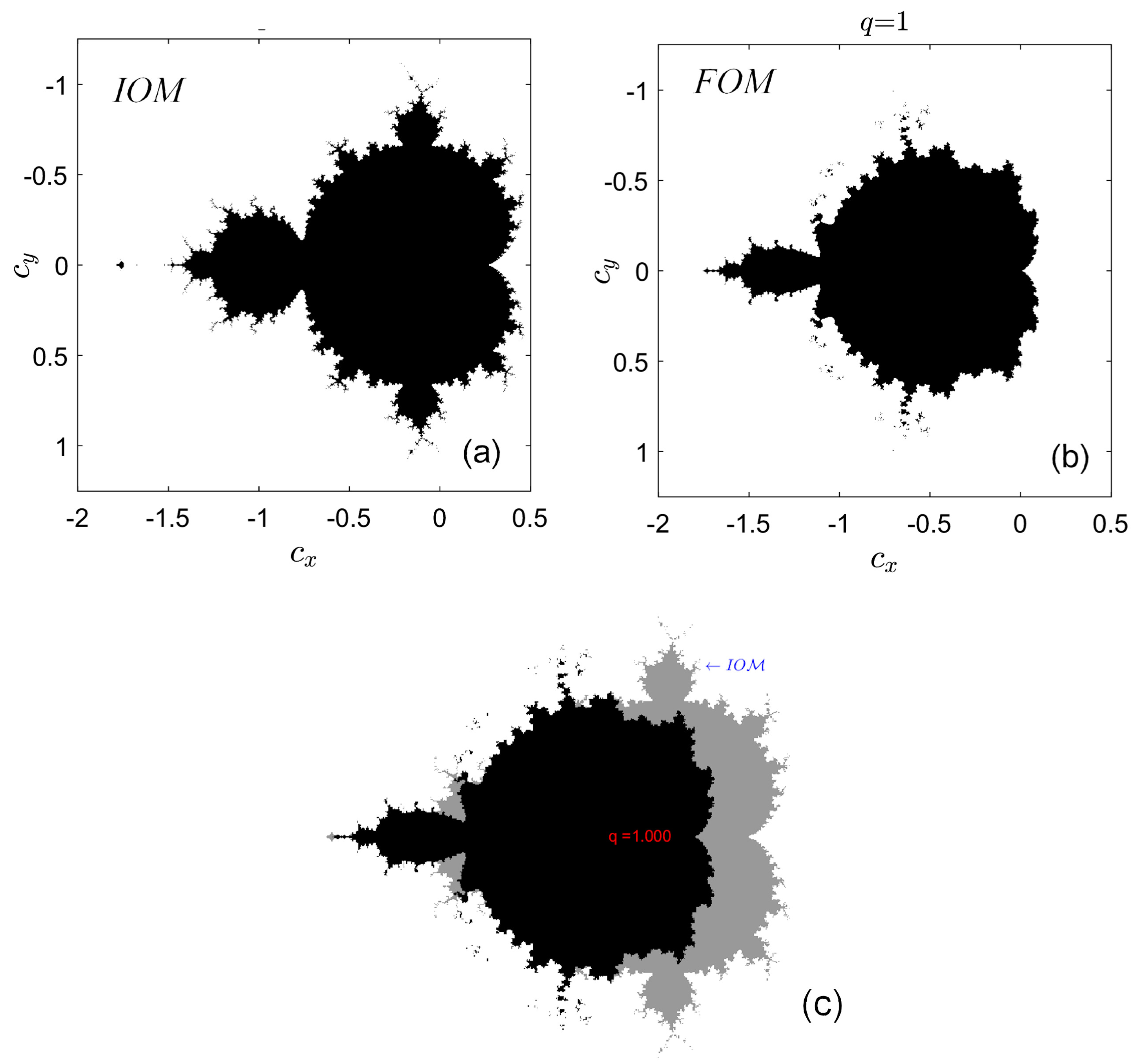
For $q\uparrow 1$, the $FO\mathcal{M}$ set differs from the $IO\mathcal{M}$ set.

Proof. 

Consider the limit of $z\left(n\right)$ for $q\uparrow 1$, with $z\left(0\right)=0$ in (5) rearranged as follows:

$$\underset{q\uparrow 1}{lim}{z\left(n\right)=z\left(n\right)|}_{q=1}=\frac{1}{\Gamma \left(q\right)}\sum _{i=1}^n\frac{\Gamma (n-i+q)}{\Gamma (n-i+1)}{|}_{q=1}{f}_c\left(z(i-1)\right)=\sum _{i=1}^n{f}_c\left(z(i-1)\right),$$

or, in a simplified form,

$$z\left(n\right)=\sum _{i=1}^n{f}_c\left(z(i-1)\right);$$

i.e., for $q\uparrow 1$, the $FO\mathcal{M}$ map generates a set different from the $IO\mathcal{M}$ set. □

The difference revealed by Proposition 3 can be viewed in Figure 4, where the $IO\mathcal{M}$ set and $FO\mathcal{M}$ set, for $q=1$, are presented.

5. Equipotential Lines and External Rays

5.1. Basic Notions on Equipotential Lines and External Rays for $IO\mathcal{M}$ and $IO{\mathcal{K}}_c$ Sets

The external arguments theory of the $IO\mathcal{M}$ set has been developed in [40,41] and popularized in [13] and makes use of an analogy to electrodynamics. It was shown that the exterior of the $IO\mathcal{M}$ set can be viewed as an electrostatic field. Consider, as described in [11,40,41], a capacitor made of a hollow metallic cylinder with a great diameter inside of which an axis of aluminum is shaped in such a way that its cross section is the Mandelbrot set. The ensembles of a cylinder and axial bar are supposed to be infinitely long. In other words, one has an aluminum bar with the cross section being the Mandelbrot set, situated in the middle of a large hollow metallic cylinder. If the interior bar is set at potential 0 and the exterior cylinder at a high potential, between the two metallic pieces appears an electric field that creates surfaces in the surrounding space. If one considers an orthogonal section through this ensemble of metallic corps and equipotential surfaces, one obtains the $IO\mathcal{M}$ set, surrounded by equipotential curves (lemniscates), sections through the equipotential surfaces with constant potential. It has been proved that the equipotential lines are also lines of equal escape time in the time escape algorithm to generate the $IO\mathcal{M}$ or $IO{\mathcal{K}}_c$ sets [11].

A particle starting from the frontier of the $IO\mathcal{M}$ set will reach the great circle surrounding the $IO\mathcal{M}$ set by following the external rays, a perpendicular curve on the equipotential lines, being gradient lines of potential.

The equipotential curves are given by

$$\underset{n\to \infty }{lim}\frac{1}{2^n}log\left|f_c^n\left(z\right)\right|,$$

(7)

while the external rays are defined as follows:

$$\underset{n\to \infty }{lim}\frac{1}{2^n}arg\left(f_c^n\left(z\right)\right),$$

(8)

where, for the Mandelbrot map, $f_c\left(z\right)=z^2+c$, one has $f^0\left(c\right)=c$, $f_c^1\left(c\right)=c^2+c$,...,$f_c^n\left(c\right)={\left(f_c^{n-1}\right)}^2+c$,...,$n=1,2,\dots$

Using the Green’s function, the Douady–Hubbard potential $U\left(c\right)$ of a point c situated between the cylinder and the outside of the Mandelbrot set can be written [42,43] (see (7)) as

$$U\left(c\right)=log|c|+\sum _{n=1}^{\infty }\frac{1}{2^n}log|1+\frac{c}{{\left[f_c^{n-1}\left(c\right)\right]}^2}|.$$

$U\left(c\right)$ is zero at points c belonging to the boundary of the $IO\mathcal{M}$ set, while for a large c, $U\left(c\right)$ is approximated by $log\left(c\right)$.

An equipotential line defined by a constant $\overline{c}\in [2,\infty )$ is a closed curve surrounding the $IO\mathcal{M}$ set and is defined as the set of points c with the property $\left\{c\right|U\left(c\right)=\overline{c}\}$, i.e., the set

$$\left\{c|log|c|+\sum _{n=1}^{\infty }\frac{1}{2^n}log|1+\frac{c}{{\left[f_c^{n-1}\left(c\right)\right]}^2}|=\overline{c}\right\}$$

The external argument $\theta \left(c\right)$ of an external ray that passes through a point c, with a large $\left|c\right|$, and which determines the point where it reaches the great circle, is the argument of the function $\Phi \left(c\right)$ given as follows [44]:

$$\Phi \left(c\right)=c\prod _{n=1}^{\infty }{\left[1+\frac{c}{{\left[f_c^{n-1}\left(c\right)\right]}^2}\right]}^{2^{-n}}.$$

The external argument of $\Phi \left(c\right)$ is (see (8))

$$\theta \left(c\right)=arg\left(c\right)+\sum _{n=1}^{\infty }\frac{1}{2^n}arg\left[1+\frac{c}{{\left[f_c^{n-1}\left(c\right)\right]}^2}\right],$$

and therefore, the external ray for a fixed angle $\overline{\theta }\in [0,2\pi )$ is the locus of points c in the complex plane that have all the same external argument with the property $\left\{c\right|\theta \left(c\right)=\overline{\theta }\}$, i.e., the set

$$\left\{c|arg\left(c\right)+\sum _{n=1}^{\infty }\frac{1}{2^n}arg\left[1+\frac{c}{{\left[f_c^{n-1}\left(c\right)\right]}^2}\right]=\overline{\theta }\right\}.$$

(9)

By $arg\left(c\right)\in [0,2\pi )$ is denoted the principal value of the argument of a complex number. To every point on the frontier of the $IO\mathcal{M}$ set, there could exist several external rays.

5.1.1. Approximations of Equipotential Lines and External Rays

Generating computationally equipotential curves and external rays using the above relations is quite a hard task. However, there exist several other simpler methods that can be applied to both the $IO\mathcal{M}$ set and the $IO{\mathcal{K}}_c$ sets.

• In [13], the potential $U\left(c\right)$ is approximated by the value $\overline{U}\left(c\right)$ defined as follows: if $|z_n|>M$, while $f_c$ is iterated, where M is, e.g., 10,000 [13], the potential can be approximated by $\overline{U}\left(c\right)\approx log\left|z_n\right|/2^n$; otherwise, if $|z_n|$ remains smaller than M, the potential is set to 0. If, for a considered constant $\overline{c}$, $\overline{U}\left(c\right)$ is close or equal to $\overline{c}$, then c, or $z_0$ in the case of Julia sets, belongs to the equipotential line, and the point c, or $z_0$, is plotted.
  An even simpler method is the level set method (LSM [13]), which, to a point c, or $z_0$, within a complex lattice, attributes a color (e.g., black), depending on the number of iterations of $f_c$ for which $|z_n|$ remains bounded. Therefore, for each $n\in [1,N]$, one obtains a level set that is approximately identical to an equipotential line.
• On the other side, the external rays (9) can be approximated by the binary decomposition method (BDM [13]) with respect to the fixed angle ${\alpha }_0\in [0,2\pi )$. Thus, to a point c, or $z_0$, within a complex lattice, one attributes a color (e.g., black or white) if the argument of $z_n$, $arg\left(z_n\right)$, belongs or does not belong to the intervals $2^n{\alpha }_0\le arg\left(z_n\right)\le 2^n{\alpha }_0+\pi (mod2\pi )$.

Drawing precisely from an external ray, e.g., inside a detail of an $IO\mathcal{M}$ or $FO\mathcal{M}$ set, is strongly restricted by the number of bits of the floating-point arithmetic used by the computer program [42]. Therefore, the external rays cannot be drawn in certain details with computer programs (see, e.g., [45]) using the double 64-bit format. Additionally, deep studies of external arguments require external arguments measured not in radians, but as fractions of complete turns. Using this unit, most of the notable points of the Mandelbrot set boundary have rational external arguments [42,43].

5.2. Equipotential Lines and External Rays of $FO\mathcal{M}$ and $FO{\mathcal{K}}_c$ Sets

The external rays for rational angles land on the frontier of the $IO\mathcal{M}$ set and connected $IO{\mathcal{K}}_c$ sets, and as verified numerically in this paper, this property holds for FO sets too.

Because writing analogue expressions of equipotential lines (7) and external rays (8) for the $FO\mathcal{M}$ or $FO{\mathcal{K}}_c$ maps, fractional equipotential lines (FELs) and fractional external rays (FERs), represents a difficult task, a possible solution is to adapt the approximations given in Section 5.1.1, where $z_n$ is used instead $f_c^n$.

In Figure 5a are presented the FELs of the $IO\mathcal{M}$ set and the $FO\mathcal{M}$ set for $q={10}^{-6}$ (see Property 1), and in Figure 5b,c are presented the FELs for $FO\mathcal{M}$ sets for $q=1$ and $q=0.5$, respectively.

As known, the following property of equipotential holds:

Proposition 4.

Equipotential lines cannot intersect each other.

While for the $IO\mathcal{M}$ set and the $FO\mathcal{M}$ set, for $q=1$, this property is obviously verified computationally (Figure 5a), for the $FO\mathcal{M}$ set with $q<1$, this property seems to be no longer verified and the FELs intersect (see Figure 5b,c).

Similarly, the FELs of $FO{\mathcal{K}}_c$ sets seem to intersect (see Figure 5d–f, where the $FO{\mathcal{K}}_c$ sets are determined for $q=0.5$ and correspond to c, chosen at the points denoted as A, B, and C in the $FO\mathcal{M}$ set in Figure 5c).

To draw FERs, one divided the complex plane $\mathbb{C}$ into sectors, where we set the same color if $\theta$ is within some certain interval [46]. Another simple way to identify the external rays is to use the ordinary escape iterations algorithm with a large escape radius and plot those points c for which $\Im \left(z_n\right)>0$. In Figure 6a are presented as overplot the FERs for the $IO\mathcal{M}$ set and the $FO\mathcal{M}$ set for $q={10}^{-6}$; in Figure 6b,c are shown the FERs for $FO\mathcal{M}$ sets with $q=1$ and $q=0.5$, respectively; and in Figure 6d–f are drawn the FERs for $FO{\mathcal{K}}_c$ sets corresponding to the points A, B, and C taken in the $FO\mathcal{M}$ set in Figure 5c.

6. Conclusions

The paper shows analytically and computationally that the Mandelbrot set of integer order can be generated as a particular case of Julia sets of Caputo-like fractional order. Moreover, it is proved that the integer-order Mandelbrot set is not a particular case of the fractional-order Mandelbrot set for the fractional order $q=1$, but only for $q\downarrow 0$. Further, the integer-order Mandelbrot set is the fractional-order Julia set for $c\downarrow 0$ and $c=0$. Additionally, the algorithms for drawing equipotential lines and external rays of a Mandelbrot set and Julia sets of integer order are adapted for a fractional-order Mandelbrot set and Julia sets. It was observed that, contrary to the integer-order case, some of these lines cross.

References

- Danca, M.-F.; Fečkan, M. Mandelbrot set and Julia sets of fractional order, M. Nonlinear Dyn. 2023, 111, 9555–9570. [Google Scholar] [CrossRef]
- Elsadany, A.A.; Aldurayhim, A.; Agiza, H.N.; Elsonbaty, A. On the Fractional-Order Complex Cosine Map: Fractal Analysis, Julia Set Control and Synchronization. Mathematics 2023, 11, 727. [Google Scholar] [CrossRef]
- Fečkan, M.; Danca, M.-F. Non-Periodicity of Complex Caputo Like Fractional Differences. Fractal Fract. 2023, 7, 68. [Google Scholar] [CrossRef]
- Danca, M.-F. On the Stability Domain of a Class of Linear Systems of Fractional Order. Fractal Fract. 2023, 7, 49. [Google Scholar] [CrossRef]
- Wang, Y.; Li, X.; Wang, D.; Liu, S. A brief note on fractal dynamics of fractional Mandelbrot sets. Appl. Math. Comput. 2022, 432, 127353. [Google Scholar] [CrossRef]
- Brooks, R.; Matelski, P. Riemann Surfaces and Related Topics: Proceedings of the 1978 Stony Brook Conference; The dynamics of 2-Generator Subgroups of PSL(2,C)Princeton University Press: Princeton, NJ, USA, 1981. [Google Scholar]
- Mandelbrot, B. Fractal Aspects of the Iteration of z↦z(1 − z) for Complex λ,z. Ann. New York Acad. Sci. 1980, 357, 249–259. [Google Scholar] [CrossRef]
- Li, J.; Pelliciari, J.; Mazzoli, C. Scale-invariant magnetic textures in the strongly correlated oxide NdNiO3. Nat. Commun. 2019, 10, 4568. [Google Scholar] [CrossRef]
- Gaston, J. Mémoire sur l’itération des fonctions rationnelles. J. Math. Pures Appl. 1918, 1, 47–245. (In French) [Google Scholar]
- Patou, P. Sur les substitutions rationnelles. Comptes Rendus Acad. Sci. Paris. 1917, 164, 806–808. [Google Scholar]
- Peitgen, H.-O.; Peter, H.R. The Beauty of Fractals Images of Complex Dynamical Systems; Springer: Berlin/Heidelberg, Germany, 1986. [Google Scholar]
- Branner, B. The Mandelbrot Set. Devaney, R.L., Keen, L., Eds.; In Chaos and Fractals: The Mathematics Behind the Computer Graphics (Proceedings of Symposia in Applied Mathematics, 39); American Mathematical Society: Providence, RI, USA, 1989; Volume 39, pp. 75–105. [Google Scholar]
- Barnsley, M.F.; Devaney, R.L.; Mandelbrot, B.B.; Peitgen, H.O.; Saupe, D.; Voss, R.F. With Contributions by Yuval Fisher Michael McGuire: The Science of Fractal Image; Springer: New York, NY, USA, 1988. [Google Scholar]
- Mandelbrot, B. The Fractal Geometry of Nature; W. H. Freeman: New York, NY, USA, 1983. [Google Scholar]
- Douady, A.; Hubbard, J.H. Etude Dynamique des Polynômes Complexes. Prépublications mathémathiques d’Orsay; Université de Paris-Sud: Paris, France, 1984. [Google Scholar]
- Kahn, J. The Mandelbrot Set is Connected: A Topological Proof. 2001. Available online: http://www.math.brown.edu/~kahn/mconn.pdf (accessed on 14 January 2024).
- Devaney, R. The Mandelbrot Set and the Farey Tree, and the Fibonacci Sequence. Amer. Math. Mon. 1999, 106, 289–302. [Google Scholar] [CrossRef]
- Magin, R.L.; Ovadia, M. Modeling the cardiac tissue electrode interface using fractional calculus. Vibr. Control. 2008, 14, 1431–1442. [Google Scholar] [CrossRef]
- Heymans, N. Dynamic measurements in long-memory materials: Fractional calculus evaluation of approach to steady state. J. Vibr. Control. 2008, 14, 1587–1596. [Google Scholar] [CrossRef]
- Lima, M.F.M.; Machado, J.A.T.; Crisóstomo, M. Experimental signal analysis of robot impacts in a fractional calculus perspective. J. Adv. Comput. Intell. Intell. Informatics 2007, 11, 1079–1085. [Google Scholar] [CrossRef]
- Debnath, L. Recent applications of fractional calculus to science and engineering. Int. J. Math. Math. Sci. 2003, 54, 3413–3442. [Google Scholar] [CrossRef]
- Huang, L.; Park, J.H.; Wu, G.C.; Mo, Z.W. Variable-order fractional discrete-time recurrent neural networks. J. Comput. App. Math. 2020, 370, 112633. [Google Scholar] [CrossRef]
- Wu, G.C. Baleanu; D. Lin, Z.X. Image encryption technique based on fractional chaotic time series. J. Vibr. Contr. 2016, 22, 2092–2099. [Google Scholar] [CrossRef]
- Abdeljawad, T.; Banerjee, S.; Wu, G.C. Discrete tempered fractional calculus for new chaotic systems with short memory and image encryption. Optik 2020, 203, 163698. [Google Scholar] [CrossRef]
- Huang, C.; Wang, J.; Chen, X.; Cao, J. Bifurcations in a fractional-order BAM neural network with four different delays. Neural Netw. 2021, 141, 344–354. [Google Scholar] [CrossRef]
- Diaz, J.B.; Olser, T.J. Differences of Fractional Order. Math. Comput. 1974, 28, 185–202. [Google Scholar] [CrossRef]
- Abdeljawad, T. On Riemann and Caputo Fractional Differences. Comput. Math. Appl. 2011, 62, 1602–1611. [Google Scholar] [CrossRef]
- Fečkan, M.; Pospíšil, M.; Danca, M.-F.; Wang, J. Caputo Delta Weakly Fractional Difference Equations. Fract. Calc. Appl. Anal. 2022, 25, 2222–2240. [Google Scholar] [CrossRef]
- Atici, F.M.; Eloe, P.W. Initial Value Problems in Discrete Fractional Calculus. Proc. Amer. Math. 2009, 137, 981–989. [Google Scholar] [CrossRef]
- Cermak, J.; Gyori, I.; Nechvatal, L. On Explicit Stability Conditions for a Linear Fractional Difference System. Fract. Calc. Appl. Anal. 2015, 18, 651–672. [Google Scholar] [CrossRef]
- Chen, F.L. A review of Existence and Stability Results for Discrete Fractional Equations. J. Comput. Complex Appl. 2015, 1, 22–53. [Google Scholar]
- Danca, M.-F. Fractional order logistic map: Numerical approach. Chaos, Solitons Fract. 2022, 157, 111851. [Google Scholar] [CrossRef]
- Diblík, J.; Fečkan, M.; Pospíšil, M. Nonexistence of Periodic Solutions and S-Asymptotically Periodic Solutions in Fractional Difference Equations. Appl. Math. Comp. 2015, 257, 230–240. [Google Scholar] [CrossRef]
- Mandelbrot Set. Available online: https://www.math.univ-toulouse.fr/~cheritat/wiki-draw/index.php/Mandelbrot_set (accessed on 12 January 2024).
- Milnor, J. Dynamics in One Complex Variable, 3rd ed.; Princeton University Press: Princeton, NJ, USA, 2006; AM-160. [Google Scholar]
- Anastassiou, G. Principles of Delta Fractional Calculus on Time Scales and Inequalities. Math. Comput. Model. 2010, 52, 556–566. [Google Scholar] [CrossRef]
- Agarwal, R.P.; Bohner, M. Basic Calculus on Time Scales and Some of its Applications. Results Math. 1999, 35, 3–22. [Google Scholar] [CrossRef]
- FO_mandelbrot. Available online: https://www.mathworks.com/matlabcentral/fileexchange/121632-fo_mandelbrot (accessed on 1 January 2024).
- Danca, M.-F.; Kuznetsov, N. D3 Dihedral Logistic Map of Fractional Order. Mathematics 2022, 10, 213. [Google Scholar] [CrossRef]
- Douady, A.; Hubbard, J.H. Itération des Polynômes Quadratiques Complexes; Académie des Sciences: Paris, France, 1982; Volume 294, pp. 123–126, Comptes Rendus des Séances de l’Académie des Sciences: Série I. Mathématique; (accessed on 12 January 2024). [Google Scholar]
- Douady, A. Algorithms for computing angles in the Mandelbrot set. Barnsley, M., Demko, S.G., Eds.; In Chaotic Dynamics and Fractals; Academic Press: New York, NY, USA, 1986; Volume 2, pp. 155–168. [Google Scholar]
- Pastor, G.; Romera, M.; Álvarez, G.; Montoya, F. Operating with external arguments in the Mandelbrot set antenna. Physica D 2002, 171, 52–71. [Google Scholar] [CrossRef]
- Romera, M.; Pastor, G.; Orue, A.B.; Martin, A.; Danca, M.-F.; Montoya, F. A Method to Solve the Limitations in Drawing External Rays of the Mandelbrot Set. Math. Probl. Eng. 2013, 2013, 105283. [Google Scholar] [CrossRef]
- Carleson, L.; Gamelin, T.W. Complex Dynamics; Springer: New York, NY, USA, 1993; p. 139. [Google Scholar]
- Jung, W. Mandel: Software for Real and Complex Dynamics. 2012. Available online: http://www.mndynamics.com/indexp.html (accessed on 12 January 2024).
- De Jong, T.G. Dynamics of Chaotic Systems and Fractals. Bachelor’s Thesis, University of Groningen, Groningen, The Netherlands, 2009. [Google Scholar]
Figure 1.
(a) set, (b) zoomed detail of zone C of the set, (c) set corresponding to (point A exterior to the set), and (d) set corresponding to (point B from the interior of the set).
Figure 2.
(a) set for ; (b) set for ; (c) set for and (see point A in Figure 2b); (d) set for corresponding to (see point B in Figure 2b); (e) set for corresponding to (see point C in Figure 2b); and (f) set for .
Figure 3.
(a) The set for and is identical to the set; (b) the set for .
Figure 4.
Differences between the set (a) and the set for (b); (c) overplot of the set and the set for (image from the animated video).
Figure 5.
(a–c) FELs of three sets for , , and , respectively; (d–f) FELs of for , corresponding to points A, B, and C from , respectively.
Figure 6.
(a–c) FERs of three sets for , , and , respectively; (d–f) FERs of three sets corresponding to points A, B, and C (Figure 5c).
Disclaimer/Publisher’s Note: The statements, opinions and data contained in all publications are solely those of the individual author(s) and contributor(s) and not of MDPI and/or the editor(s). MDPI and/or the editor(s) disclaim responsibility for any injury to people or property resulting from any ideas, methods, instructions or products referred to in the content. |
© 2024 by the author. Licensee MDPI, Basel, Switzerland. This article is an open access article distributed under the terms and conditions of the Creative Commons Attribution (CC BY) license (https://creativecommons.org/licenses/by/4.0/).
Share and Cite
MDPI and ACS Style
Danca, M.-F. Mandelbrot Set as a Particular Julia Set of Fractional Order, Equipotential Lines and External Rays of Mandelbrot and Julia Sets of Fractional Order. Fractal Fract. 2024, 8, 69. https://doi.org/10.3390/fractalfract8010069
AMA Style
Danca M-F. Mandelbrot Set as a Particular Julia Set of Fractional Order, Equipotential Lines and External Rays of Mandelbrot and Julia Sets of Fractional Order. Fractal and Fractional. 2024; 8(1):69. https://doi.org/10.3390/fractalfract8010069
Chicago/Turabian StyleDanca, Marius-F. 2024. "Mandelbrot Set as a Particular Julia Set of Fractional Order, Equipotential Lines and External Rays of Mandelbrot and Julia Sets of Fractional Order" Fractal and Fractional 8, no. 1: 69. https://doi.org/10.3390/fractalfract8010069